Avant d'utiliser un marqueur (une fois qu'on a vérifié qu'il est bien polymorphe), il convient de s'assurer qu'on observe bien les proportions mendéliennes auxquelles on s'attend, à l'aide d'un test du Chi2.
Dans une expérience, on constate les effectifs suivants dans la génération F2.
A:  7
B: 12
H: 20
Ces effectifs sont-ils semblables à ce à quoi on pouvait s'attendre ?
> chisq.test(c(7,12,20),p=c(.25,.25,.5))
      Chi-squared test for given probabilities
data:  c(7, 12, 20)
X-squared = 1.3077, df = 2, p-value = 0.52
Oui.
Idem :
> chisq.test(c(10,4,23),p=c(.25,.25,.5))
      Chi-squared test for given probabilities
data:  c(10, 4, 23)
X-squared = 4.1351, df = 2, p-value = 0.1265
Dans une expérience avec des lignées recombinantes, on trouve les phénotypes suivants :
A:   15
B:   12
H:    6
Ces quantités sont-elles semblables à ce à quoi on pouvait s'attendre ?
# On ne tient pas compte des hétérozygotes
> chisq.test(c(15,12))
      Chi-squared test for given probabilities
data:  c(15, 12)
X-squared = 0.3333, df = 1, p-value = 0.5637
Oui.
huile.BB <- c(40.74, 34.9, 33.5, 33.4, 36.47, 31.5, 36.7, 36, 37.22,
37.1, 38.64, 34.97, 31.78, 37.98, 38.75, NA, 31.45, 45.98, 37.76,
38.61, 36.38, 36.75, 35.4, 41.65, 42.63, 36.57, 40.5, 34.8, 32.55,
36.3, 37.23, 33.9, 36.36, 36.24, 36.35, 39.95, 35.53, 36.4, 39.58,
43.3, 36.98, 40.34, NA, 34.65, 34.44, 37.12, 38.4, 38.43, 32.3,
35.06, 33.7, 34.58, 35.98, 38.3, 38.67)
huile.Bb <- c(40.04, 35.65, 39, 38.16, 33.7, 37.5, 38.98, 41.2,
36.37, 40.6, 35.2, 40, 35.63, 34.02, 32.6, 37.8, 40, 33.8, 42.6,
42.6, 41.92, 43.3, 36.7, 33.25, 37.86, 40.8, 35.63, 37.98, 36.05,
36.53, 38.92, 42.54, 40.6, 40.32, 34.3, 35.9, 41.75, 40.33, 44.4,
42.55, 42.22, 39.6, 42.76, NA, 43.17, 39.5, 40.2, 34.58, 40.75,
43.54, 32.93, 43.84, 39.9, 39.03, 41.43, 39.03, 35.94, 39.43, 37.7,
37.2, 42.38, 36.75, 39.12, 42.75, 45.64, 48.9, 41.3, 38.8, 43.58,
36.63, 39.75, 46.8, 47.82, 34.48, 41.26, 42.43, 43.26, 35.22, 40.05,
37.28, 37.26, 36, 37.98, 37.52, 41.22, 32, 38.25, 40.24, 38.3,
42.34, 45.57, 37.84, 38.38, 46.6, 38.94, 40.56, 45.6, 40.7, 33.9,
39.7, 43.7, 35.83, 37.38, 41.85, 41.93, 40.28, 39.68, 38.88, 45.38,
41.72, 39.8, 40.03, 49.7, 37.57, 46.8, 46.07, 44.78, 40.35, 36.88,
32.05, 38.02, 30.17, 34.9, 39.14)
huile.bb <- c(46.3, 41.8, 47.6, 45.53, 42.88, 45.47, 49.06, 49.05,
46.2, 40.1, 47.58, 44.63, 51.45, 42.93, 50.2, 45.27, 43.03, 48.34,
50.3, 41.53, 46, 47.3, 50.4, 49.48, 47.46, 48.15, 41.02, 46.85,
37.93, 48.17, 42.93, 51.58, 42.94, 42.34, 46.3, 41.45, 49.62, 44.15,
41.9, 45.26, 50.42)
attaques.BB <- c(85.75, 70.09, 69.59, 74.31, 97.37, 79.24, 60.54,
44.07, 46.5, 63.83, 51.06, 89.49, 90, 66.15, 90, 73.58, 75.13,
66.03, 31.48, 94.23, 95.92, 92.65, 90, 62.06, 72.9, 89.77, 87.73,
86.85, 74.43, 68.97, 57.69, 86, 52.31, 66.15, 61.84, 85.81, 98.21,
71.94, 41.95, 88.1, 78.47, 46.31, 73.75, 96, 67.5, 98.08, 93.75,
83.92, 96.67, 92.86, 91.67, 81.25, 94.12, 89.97, 89.47)
attaques.Bb <- c(50, 75.36, 69.66, 74.37, 82.05, 86.31, 52.38,
47.65, 79.17, 77.3, 51.81, 71.79, 70.08, 69.41, 32.82, 55.65, 64.04,
64.07, 32.16, 49.31, 53.51, 31.29, 38.41, 79.17, 70.33, 60.1, 43.57,
23.57, 14.08, 78.46, 47.73, 35.93, 67.92, 68.75, 35.91, 5.95, 40.57,
64.46, 76.45, 61.54, 40.38, 74.48, 18.04, 88.23, 80.36, 46.3, 58.79,
67.39, 24.74, 80.64, 40.8, 77.08, 78.85, 87.98, 74.37, 86.41, 66.58,
88.83, 81.03, 68.52, 28.87, 97.73, 30.06, 70.54, 34.49, 48.33,
90.43, 49.42, 83.33, 86.23, 53.85, 70.69, 36.7, 42, 52.92, 79.27,
71.82, 48.53, 36.79, 84.46, 26.59, 57, 57.64, 62.93, 56.64, 67.46,
22.02, 33.97, 43.73, 68.61, 84.23, 66.58, 72.02, 14.29, 58.33,
44.58, 76, 75.05, 48.18, 53.23, 62.22, 69.38, 88.05, 76, 91.81,
56.36, 84.52, 54.83, 78.13, 92.11, 75.83, 50, 77.08, 70.54, 68.68,
75, 74.89, 39.6, 75.71, 75.39, 62.5, 58.82, 78.71, 65.63)
attaques.bb <- c(84.74, 80.59, 61.81, 46, 66.69, 37.63, 33.69,
27.08, 88.15, 25, 71.72, 56.74, 39.13, 29.26, 93.75, 28.22, 70.69,
60, 41.43, 42.31, 54.26, 45.23, 57.91, 68.75, 79.17, 73.75, 16.67,
69.08, 42.68, 47.62, 60.09, 70, 75.83, 72.26, 82.11, 73.75, 89.29,
35, 46.65, 82.21, 62.14)
poids.BB <- c(22.02, 14.96, 15.65, 19.7, 9.48, 6.44, 13.18, 7.06,
37.2, 9.94, 11.42, 5.56, 18, 28.2, 12.34, 0.72, 21.55, 24.4, 23.78,
13.48, 16.38, 8.1, 5.2, 13, 19.94, 5.94, 15.46, 2.45, 6.32, 14.98,
12.04, 35.58, 20.84, 28.62, 13.68, 29.74, 14.65, 18.16, 6.92, 11.73,
16.18, 23.8, 2.1, 6.04, 11.78, 15.16, 11.3, 15.84, 16.88, 25, 10.14,
19.16, 17.74, 9.2, 15.25)
poids.Bb <- c(14.02, 13.14, 8.58, 34.4, 18.08, 8.98, 13.96, 9.32, 16.1,
8.25, 16.08, 24.2, 7.34, 28.9, 9.5, 13.06, 20.66, 16.8, 5.65, 13.8,
10.34, 16.8, 9.7, 13.1, 19.28, 13.86, 10.44, 10.56, 11.46, 11.03,
23.9, 11.96, 9, 13.42, 9.56, 11.58, 3.38, 17.06, 31.38, 16.05, 8.74,
9.48, 26.34, 6.43, 8.7, 13.86, 20.76, 13.36, 10.7, 12.18, 12.04,
31.16, 26.84, 14.18, 14.3, 10.78, 12.2, 12.52, 33.06, 20.46, 11.86,
17.56, 24.78, 13.24, 13.78, 5.62, 18.34, 6.04, 20.26, 8.44, 9.08,
11.62, 11.52, 11.06, 16.42, 14.12, 16.92, 24.74, 22.85, 11.02,
14.54, 26.18, 20.78, 18.08, 13.52, 16.86, 11.25, 10.68, 19.78,
28.88, 11.46, 15.28, 30.46, 6.9, 20.64, 17.84, 14.78, 3.6, 5.96,
14.03, 10.54, 10.36, 12.68, 14.72, 5.68, 20.1, 20.76, 17.6, 21.8,
31.88, 13.96, 10.14, 5.04, 6.46, 3.43, 13.43, 7.32, 5.76, 14.86,
10.94, 25.2, 10.24, 17.9, 20.82)
poids.bb <- c(11.3, 3.84, 4.84, 7.36, 10.16, 7.12, 10.56, 6.88, 9.56,
5.86, 14.2, 8.64, 7.62, 4.65, 7.56, 7.5, 12.05, 12.48, 6.96, 10.38,
16.3, 13.64, 14.68, 14.56, 11.96, 16.55, 7.88, 4.65, 14.17, 16.1,
4.72, 10.9, 11.82, 13.48, 5.42, 3.3, 12.2, 7.35, 9.04, 17.24, 18.3)
d1 <- data.frame(
phenotype=c(attaques.BB,attaques.Bb,attaques.bb),
genotype=c(rep("BB",length(attaques.BB)),
rep("Bb",length(attaques.Bb)),
rep("bb",length(attaques.bb))))
d2 <- data.frame(
phenotype=c(huile.BB,huile.Bb,huile.bb),
genotype=c(rep("BB",length(huile.BB)),
rep("Bb",length(huile.Bb)),
rep("bb",length(huile.bb))))
d3 <- data.frame(
phenotype=c(poids.BB,poids.Bb,poids.bb),
genotype=c(rep("BB",length(poids.BB)),
rep("Bb",length(poids.Bb)),
rep("bb",length(poids.bb))))
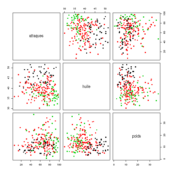
d <- data.frame(attaques=d1$phenotype,
huile=d2$phenotype,
poids=d3$phenotype,
genotype=d1$genotype)
plot(d[,1:3], col=(1:3)[d$genotype], pch=15)
draw.ellipse <- function (x, y=NULL, N=100, method=lines, ...) {
  if (is.null(y)) {
    y <- x[,2]
    x <- x[,1]
  }
  centre <- c(mean(x,na.rm=T), mean(y,na.rm=T))
  m <- matrix(c(var(x,na.rm=T),cov(x,y,use='c'),cov(x,y,use='c'),var(y,na.rm=T)),nr=2,nc=2)
  e <- eigen(m)
  r <- sqrt(e$values)
  v <- e$vectors
  theta <- seq(0,2*pi, length=N)
  x <- centre[1] + r[1]*v[1,1]*cos(theta) + r[2]*v[1,2]*sin(theta)
  y <- centre[2] + r[1]*v[2,1]*cos(theta) + r[2]*v[2,2]*sin(theta)
  method(x,y,...)
}

my.plot <- function (d, f, col=rainbow(length(levels(f))),
                     draw=draw.ellipse, ...) {
  plot(d, col=col[as.numeric(f)], pch=16, ...)
  for (i in 1:length(levels(f))) {
    try(
      draw(d[ as.numeric(f)==i, ], col=col[i])
    )
  }
  abline(h=0,lty=3)
  abline(v=0,lty=3)
  legend(par('usr')[1],par('usr')[3],xjust=0,yjust=0,
         levels(f),
         col=col,
         lty=1,lwd=3)
}

op <- par(mfrow=c(2,2))
my.plot(d[,c(1,2)], d$genotype)
plot.new()
my.plot(d[,c(1,3)], d$genotype)
my.plot(d[,c(2,3)], d$genotype)
par(op)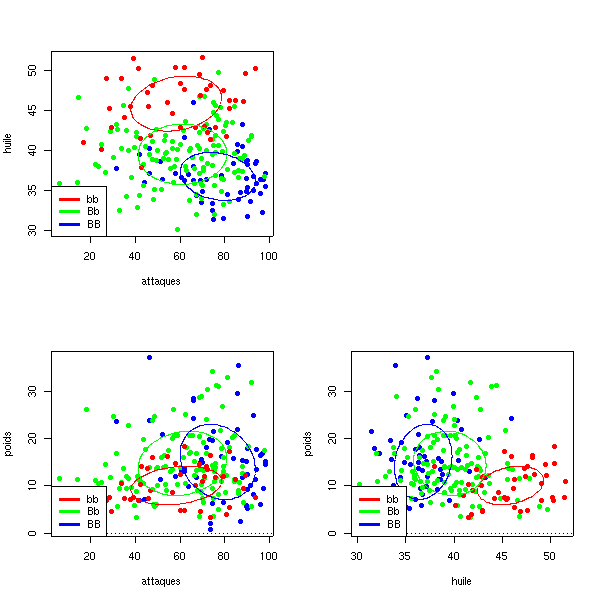
Ces graphiques suggèrent : le marqueur est lié à la résistance aux attaques et à la teneur en huile mais pas vraiment au poids du grain, le QTL "résistance aux attaques" est dominant, le QTL "teneur en huile" est plutôt additif.
1. Pour chaque QTL, regarder sa distribution. Faire éventuellement une transformation pour que les données soient gaussiennes. Les transformations les plus courrantes sont des élévations à la puissance ou le logarithme.
Pour cet exercice, on nous suggère arcsin(sqrt(p)), sqrt(p), log(p).
2. Faire une analyse de variance pour voir si le QTL est lié au marqueur qui nous intéresse.
3. Corriger la p-valeur en considérant qu'il y a 290 marqueurs sur la carte génétique.
4. Faire des tests afin de voir si le QTL (enfin, le morceau du QTL qui est proche du marqueur) est additif ou dominant.
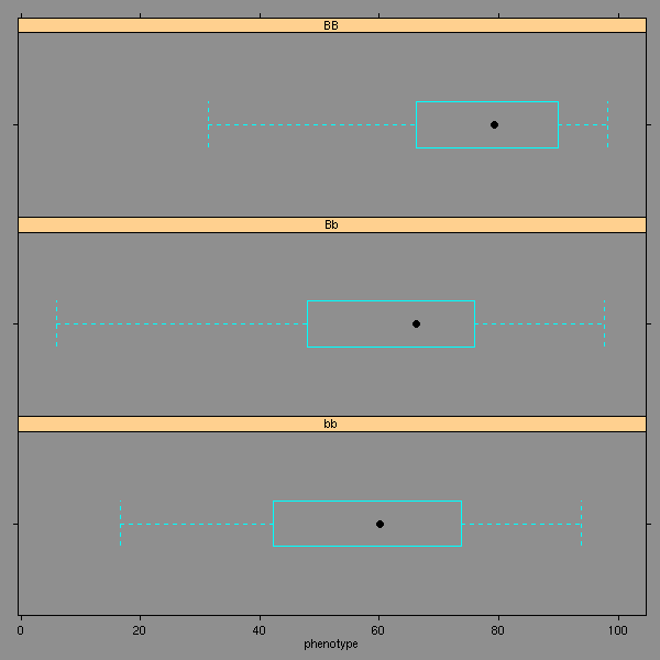
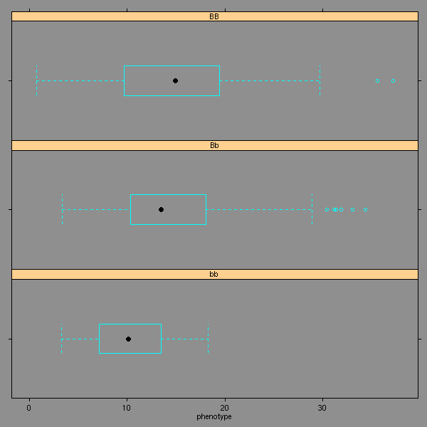
On commence par regarder les données.
library(lattice)
bwplot(~phenotype|genotype,data=d1,layout=c(1,3))
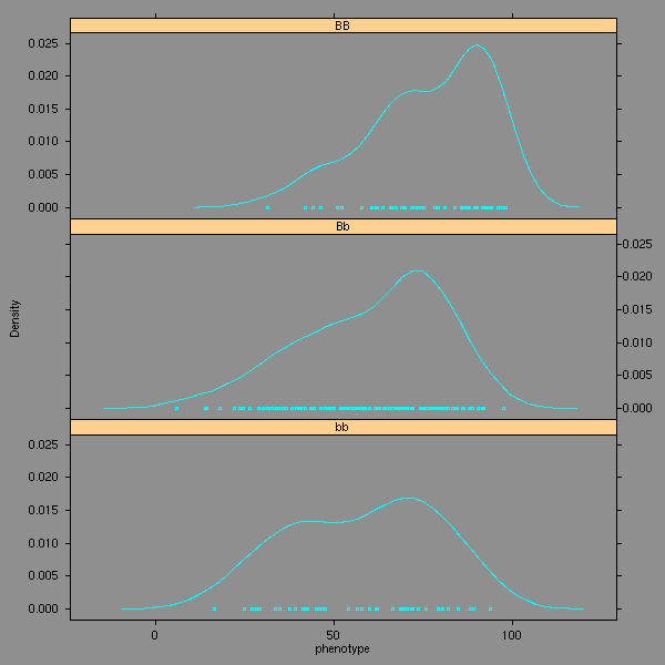
densityplot(~phenotype|genotype,data=d1,layout=c(1,3))

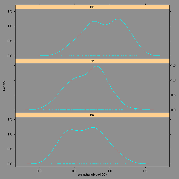
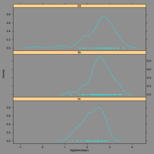
Les données ne sont visiblement pas normales. On regarde les différentes transformations qui nous sont suggérées.
densityplot(~phenotype|genotype,data=d1, layout=c(1,3))
densityplot(~sqrt(phenotype)|genotype,data=d1, layout=c(1,3))
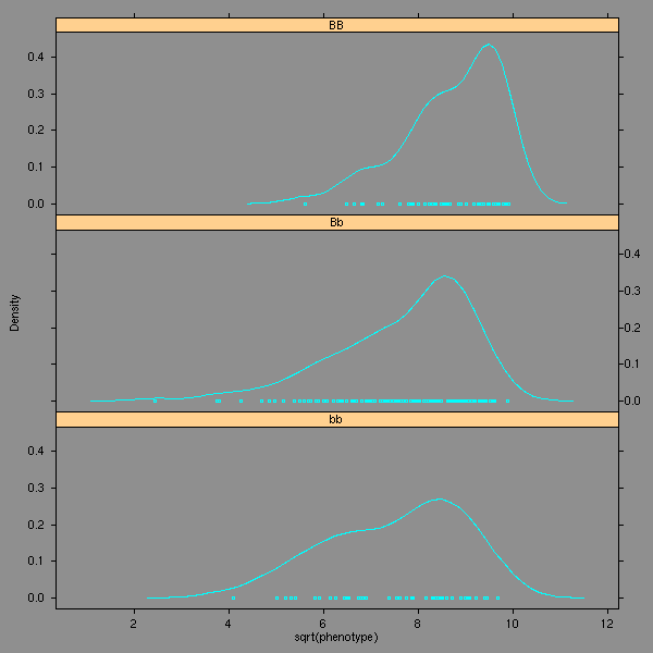
densityplot(~log(phenotype)|genotype,data=d1, layout=c(1,3))

densityplot(~asin(phenotype/100)|genotype,data=d1, layout=c(1,3))
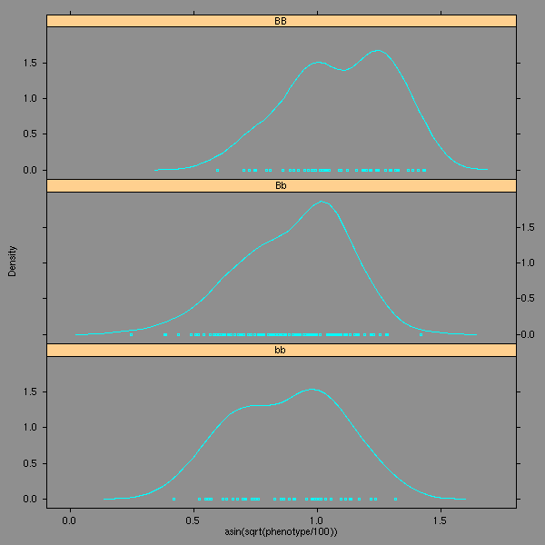
densityplot(~asin(sqrt(phenotype/100))|genotype,data=d1, layout=c(1,3))
Les graphiques quantiles/quantiles sont une autre manière de regarder la normalité d'une variable.
transformations <- c(
  function(x){x},
  function(x){sqrt(x)},
  function(x){asin(x/100)},
  function(x){asin(sqrt(x/100))},
  function(x){log(x)}
)
op <- par(mfrow=c(5,3))
for (f in transformations) {
  for (i in 1:3) {
    x <- f(d1$phenotype[d1$genotype==levels(d1$genotype)[i]])
    qqnorm(x, main=round(shapiro.test(x)$p.value,3))
    qqline(x, col='red')
  }
}
par(op)
Il y a encore une manière de regarder la normalité d'une variable : le test de Shapiro-Wilk (dont la p-valeur apparaît comme titre des diagrammes quantiles/quantiles précédents).
for (f in transformations) {
  res <- rep(NA,3)
  for (i in 1:3) {
    res[i] <- shapiro.test(f(d1$phenotype[d1$genotype==levels(d1$genotype)[i]]))$p.value
  }
  print(res)
}
Il vient :
[1] 0.267568407 0.001633154 0.002006893
[1] 1.061572e-01 2.220330e-06 3.198249e-04
[1] 0.5525346 0.4585406 0.1770722
[1] 0.7261533 0.0817244 0.1438315
[1] 1.012883e-02 1.291891e-10 2.966839e-05
On choisit donc la transformation 3 ou 4. L'énoncé nous demandait de prendre asin(sqrt(x/100)) : c'est correct, c'est ce qu'on prendra.
Avant de faire une analyse de la variance, il convient de vérifier que ses hypothèses sont bien satisfaites : nous venons de voir la normalité, il reste l'équivariance.
> bartlett.test(phenotype~genotype,data=d1)
      Bartlett test for homogeneity of variances
data:  phenotype by genotype
Bartlett's K-squared = 2.2705, df = 2, p-value = 0.3213
Pour la transformation que nous venons de choisir :
> bartlett.test(asin(sqrt(phenotype/100))~genotype,data=d1)
      Bartlett test for homogeneity of variances
data:  asin(sqrt(phenotype/100)) by genotype
Bartlett's K-squared = 0.1831, df = 2, p-value = 0.9125
On peut maintenant passer à l'analyse de la variance : le génotype (plus précisément : le marqueur dont on dispose) a-t-il un effet sur le phénotype ?
> summary(lm(asin(sqrt(phenotype/100))~genotype,data=d1))

Call:
lm(formula = asin(sqrt(phenotype/100)) ~ genotype, data = d1)

Residuals:
    Min      1Q  Median      3Q     Max
-0.6585 -0.1455  0.0274  0.1538  0.5146

Coefficients:
            Estimate Std. Error t value Pr(>|t|)
(Intercept)  0.87652    0.03380  25.933  < 2e-16 ***
genotypeBb   0.02840    0.03899   0.728    0.467
genotypeBB   0.21883    0.04465   4.900 1.87e-06 ***

Residual standard error: 0.2164 on 217 degrees of freedom
Multiple R-Squared: 0.1385,     Adjusted R-squared: 0.1305
F-statistic: 17.44 on 2 and 217 DF,  p-value: 9.486e-08
La p-valeur est de l'ordre de 10^-7 : il y a des différences notables.
Les p-valeurs données sont correctes si on ne fait qu'un seul test : c'est la probabilité qu'on rejette à tors l'hypothèse nulle.
Par contre, si on fait une multitude de tests, on aimerait avoir la probabilité de rejeter à tors l'une des hypothèses nulles.
Si on fait N tests et si on suppose qu'il sont indépendants, on remplace la p-valeur p par :
1-(1-p)^N.
(Je crois que ça s'appelle la "correction de Sidak".)
(Si les tests ne sont pas indépendants, cette p-valeur est "trop prudente".)
(On parle parfois de "correction de Bonferroni" : il s'agit de remplacer p par N*p. La correction mentionnée plus haut est plus pertinente.)
Il existe plein d'autres corrections (très utilisées pour l'analyse de résultats de puces à ADN) : sous R, voir par exemple la fonction mt.rawp2adjp de la bibliothèque multtest. Voir aussi, de manière plus générale, le projet bioconductor.
Dans notre cas :
> 1-(1-1e-7)^290
[1] 2.899958e-05
r <- lm(asin(sqrt(phenotype/100)) ~ genotype, data = d1)
r.dominant <- lm(asin(sqrt(phenotype/100)) ~
                 factor(d1$genotype %in% c('BB','Bb')), data = d1)
r.additif <- lm(asin(sqrt(phenotype/100)) ~
                ifelse(d1$genotype=="BB",1,ifelse(d1$genotype=="Bb",0,-1)), data=d1)
Le modèle complet est-il meilleur que le modèle dominant ?
>   anova(r.dominant,r)
Analysis of Variance Table

Model 1: asin(sqrt(phenotype/100)) ~ factor(d1$genotype %in% c("BB", "Bb"))
Model 2: asin(sqrt(phenotype/100)) ~ genotype
  Res.Df     RSS  Df Sum of Sq      F    Pr(>F)
1    218 11.5458
2    217 10.1642   1    1.3816 29.497 1.496e-07 ***
---
Signif. codes:  0 `***' 0.001 `**' 0.01 `*' 0.05 `.' 0.1 ` ' 1
Oui.
Le modèle complet est-il meilleur que le modèle additif ?
> anova(r.additif,r)
Analysis of Variance Table

Model 1: asin(sqrt(phenotype/100)) ~ ifelse(d1$genotype == "BB", 1, ifelse(d1$genotype ==
    "Bb", 0, -1))
Model 2: asin(sqrt(phenotype/100)) ~ genotype
  Res.Df     RSS  Df Sum of Sq      F   Pr(>F)
1    218 10.5150
2    217 10.1642   1    0.3508 7.4901 0.006718 **
Oui.
On gardera donc un modèle semi-additif.
Regardons les données :
library(lattice)
bwplot(~phenotype|genotype,data=d2,layout=c(1,3))

Normalité des données, quelques transformations :
densityplot(~phenotype|genotype,data=d2, layout=c(1,3))

densityplot(~sqrt(phenotype)|genotype,data=d2, layout=c(1,3))
densityplot(~log(phenotype)|genotype,data=d2, layout=c(1,3))

densityplot(~asin(phenotype/100)|genotype,data=d2, layout=c(1,3))

densityplot(~asin(sqrt(phenotype/100))|genotype,data=d2, layout=c(1,3))

transformations <- c(
  function(x){x},
  function(x){sqrt(x)},
  function(x){asin(x/100)},
  function(x){asin(sqrt(x/100))},
  function(x){log(x)}
)
op <- par(mfrow=c(5,3))
for (f in transformations) {
  for (i in 1:3) {
    x <- f(d2$phenotype[d2$genotype==levels(d2$genotype)[i]])
    qqnorm(x, main=round(shapiro.test(x)$p.value,3))
    qqline(x, col='red')
  }
}
par(op)
for (f in transformations) {
  res <- rep(NA,3)
  for (i in 1:3) {
    res[i] <- shapiro.test(f(d2$phenotype[d2$genotype==levels(d2$genotype)[i]]))$p.value
  }
  print(res)
}

[1] 0.3450675 0.9373818 0.2105760
[1] 0.2979586 0.9905358 0.3980080
[1] 0.3694092 0.8607130 0.1607268
[1] 0.3427520 0.9713968 0.2756805
[1] 0.2431749 0.9778920 0.6001771
On choisit de ne pas faire de transformation.
Equivariance :
> bartlett.test(phenotype~genotype,data=d2)
      Bartlett test for homogeneity of variances
data:  phenotype by genotype
Bartlett's K-squared = 3.6616, df = 2, p-value = 0.1603
Analyse de la variance :
> summary(lm(phenotype~genotype,data=d2))

Call:
lm(formula = phenotype ~ genotype, data = d2)

Residuals:
     Min       1Q   Median       3Q      Max
-9.38951 -2.29951 -0.05698  2.27439 10.14049

Coefficients:
            Estimate Std. Error t value Pr(>|t|)
(Intercept)  45.8756     0.5506  83.316   <2e-16 ***
genotypeBb   -6.3161     0.6358  -9.934   <2e-16 ***
genotypeBB   -9.0686     0.7333 -12.367   <2e-16 ***
---
Signif. codes:  0 `***' 0.001 `**' 0.01 `*' 0.05 `.' 0.1 ` ' 1

Residual standard error: 3.526 on 214 degrees of freedom
Multiple R-Squared: 0.4265,     Adjusted R-squared: 0.4211
F-statistic: 79.57 on 2 and 214 DF,  p-value: < 2.2e-16
Correction de la p-valeur :
> 1-(1-2.2e-16)^290
[1] 6.439294e-14
QTL partiellement additif :
r <- lm(phenotype ~ genotype, data = d2)
r.dominant <- lm(phenotype ~
                 factor(d2$genotype %in% c('BB','Bb')), data = d2)
r.additif <- lm(phenotype ~
                ifelse(d2$genotype=="BB",1,ifelse(d2$genotype=="Bb",0,-1)), data=d2)

> anova(r,r.dominant)
Analysis of Variance Table
Model 1: phenotype ~ genotype
Model 2: phenotype ~ factor(d2$genotype %in% c("BB", "Bb"))
  Res.Df     RSS  Df Sum of Sq      F    Pr(>F)
1    214 2660.14
2    215 2940.77  -1   -280.63 22.576 3.703e-06 ***

>  anova(r,r.additif)
Analysis of Variance Table
Model 1: phenotype ~ genotype
Model 2: phenotype ~ ifelse(d2$genotype == "BB", 1, ifelse(d2$genotype ==
    "Bb", 0, -1))
  Res.Df     RSS  Df Sum of Sq      F    Pr(>F)
1    214 2660.14
2    215 2827.72  -1   -167.58 13.481 0.0003044 ***
Regardons les données :
bwplot(~phenotype|genotype,data=d3,layout=c(1,3))
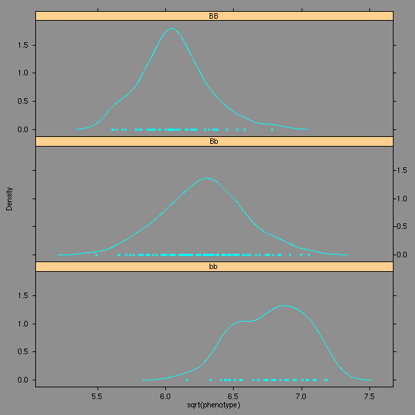
Normalité des données, quelques transformations :
densityplot(~phenotype|genotype,data=d3, layout=c(1,3))

densityplot(~sqrt(phenotype)|genotype,data=d3, layout=c(1,3))

densityplot(~log(phenotype)|genotype,data=d3, layout=c(1,3))
transformations <- c(
  function(x){x},
  function(x){sqrt(x)},
  function(x){log(x)}
)
op <- par(mfrow=c(3,3))
for (f in transformations) {
  for (i in 1:3) {
    x <- f(d3$phenotype[d3$genotype==levels(d3$genotype)[i]])
    qqnorm(x, main=round(shapiro.test(x)$p.value,3))
    qqline(x, col='red')
  }
}
par(op)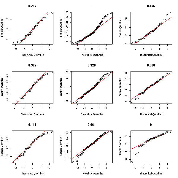
for (f in transformations) {
  res <- rep(NA,3)
  for (i in 1:3) {
    res[i] <- shapiro.test(f(d3$phenotype[d3$genotype==levels(d3$genotype)[i]]))$p.value
  }
  print(res)
}

[1] 2.170423e-01 3.717989e-05 1.452725e-01
[1] 0.3217445 0.1262890 0.8679819
[1] 0.1109250427 0.0606293629 0.0000675456
Equivariance :
for (f in transformations) {
  print(bartlett.test(f(phenotype)~genotype,data=d3)$p.value)
}

[1] 0.0001150813
[1] 0.005037395
[1] 0.0005259798
C'est très mauvais, dans tous les cas. On choisira la transformation "racine carrée", qui est la "moins pire".
Analyse de la variance :
Call:
lm(formula = sqrt(phenotype) ~ genotype, data = d3)

Residuals:
     Min       1Q   Median       3Q      Max
-2.88597 -0.52969 -0.02874  0.54184  2.36468

Coefficients:
            Estimate Std. Error t value Pr(>|t|)
(Intercept)   3.1089     0.1400  22.201  < 2e-16 ***
genotypeBb    0.6387     0.1615   3.954 0.000104 ***
genotypeBB    0.6256     0.1850   3.381 0.000855 ***
---
Signif. codes:  0 `***' 0.001 `**' 0.01 `*' 0.05 `.' 0.1 ` ' 1

Residual standard error: 0.8966 on 217 degrees of freedom
Multiple R-Squared: 0.07155,    Adjusted R-squared: 0.06299
F-statistic: 8.361 on 2 and 217 DF,  p-value: 0.0003177
Correction de la p-valeur :
> 1-(1-0.0003177)^290
[1] 0.0880295
La liaison entre le QTL et le marqueur n'est plus significative. On arrête l'analyse.
A cause du problème d'équivariance, on aurait pu faire une analyse de la variance non paramétrique, qui conduit aux mêmes conclusions :
> r <- kruskal.test(phenotype ~ genotype, data=d3)
> r
        Kruskal-Wallis rank sum test
data:  phenotype by genotype
Kruskal-Wallis chi-squared = 16.4084, df = 2, p-value = 0.0002735

> 1-(1-r$p.value)^290
[1] 0.07626181
On peut résumer tous les tests précédents dans un tableau.
                   Attaque            Huile                Poids
----------------------------------------------------------------------------
Transformation    asin(sqrt(x))       aucune               sqrt(x)
Shapiro           0.73, 0.08, 0.14    0.35, 0.94, 0.21     0.32, 0.13, 0.87
Bartlett          0.91                0.1603               0.005
Anova             1e-7                1e-16                3e-4
Anova (corrigé)   3e-5                1e-13                .09
Additif ?         1e-7                4e-6
Dominant ?        7e-3                3e-4
Les QTL "Attaque" et "Huile" sont liés au marqueur, le QTL "Poids" non.
Vincent Zoonekynd
<zoonek@math.jussieu.fr>
latest modification on Tue Feb 24 20:52:14 CET 2004