Survival analysis
Introduction
Some Models
Kaplan-Meier estimation
Discrete time models
Parametric regression models
Proportional Hazard (PH) models
Accelerated Failure Time (AFT) models
Other models
Cox Proportional Hazard model
TODO
Spatial data and GIS (Geographical Information Systems)
Bootstrap and simulations
Simulations: Parametric bootstrap
Non-parametric bootstrap
Other examples
TODO: delete what follows?
TODO
TODO
MCMC: Monte Carlo simulations with Markov Chains
Bayesian methods and MCMC
Graph theory
Linguistics
In this chapter:
Survival analysis
Spatial statistics
Bootstrap and simulations (this should be somewhere else...)
MCMC
Graph theory
TODO: finish writing this -- I have not mentionned Cox regression yet.
TODO: structure of this chapter
Survival Analysis with no predictive variables
  Survival function, Hazard function, Cumulative hazard function
  Some distributions
  Non-parametric methods: Kaplan-Meier estimation
  Oarametric methods: TODO
Discrete models
Survival Analysis with predictive variables
  TODO
TODO:
One should clearly distinguish discrete survival data and continuous
survival data.
Quite often, one only mentions continuous data and caters to
discrete data as if they were continuous -- it is a bad idea.
TODO:
Survival data are quite tricky to use: we shall replace them by
(say) the survival function. A function is easier to handle.
TODO:
Problem with classical regression: it does not allow censored data
(i.e., data of the form "more than 2" or "less that 15" or "between
2 and 15", i.e., intervals instead of numbers), nor time-dependant
predictive variables.
TODO:
No predictive variables:
- Parametric variables (MLE, with the models mentionned below)
- non parametric methods (Kaplan-Meier (continuous case)
  or LifeTable (discrete case))

With predictive variables:
- parametric methods
- semi-parametric methods (Cox regression: parametric for the part
that depends on the predictive variables, non-parametric for the
rest)
TODO: frailty = unobserved heterogeneity.
TODO: What difference between survival data and longitudinal data?
We are interested, in this chapter, in survival variables: a survival variable is very similar to a quantitative variable, but it can assume both precise numeric values, such as "13 years", but also less precise values, such as "more than 15 years".
Those less precise values are called "censored values". They are usually written as
10+    More that 10 (right censored)
5-     Less than 5 (left censored)
[5,10] Between 5 and 10
You get that kind of data, for instance, when you study the survival after a cancer: if the study lasts ten years, you will have the precise survival of the patients who died, but for the others, you will only know that they survived more than 10 years. Furthernore, some patients will have left the study (because they moved, got bored, or died in an accident): you will just know that they survived as long as they were in the study -- their survival time will also be right censored.
Left censorship corresponds to the events that took place before the study began.
TODO: give a concrete example.
You get interval censorship for instance when a symptom is first seen in a medical examination: we know it has appeared since the previous examination, but you do not know when.
Here are other examples:
survival of a patient
survival of a marriage
survival of a company
time until a machine breaks down
time until a trendy product becomes less popular and ceases to be produced
survival of a high school teacher (until his resignation, his admission in asylum, his suicide, etc.)
time until a patient stops to take a drug
etc.
You can also see survival variables as binary qualitative variables (those you try to forecast in logistic regression) indicating wether the event occurred, to which you have added the time it occurred. The censored values correspond to "the event did not occurred"; in the above examples, this is equivalent to replacing "alive/dead" by "alive / date of death".
Survival variables can have several values, for instance "healthy", "ill", "death" (and if the patient is cured between two deseases, it gets even more complicated). In more complex situations, we sometimes speak of "transitionnal data" (we are interested in the transition from one state to another) or "spell duration data".
You can also see survival data as qualitative time series, in which you are interested in the transitions from one state to another.
Time Series:
Time   1  2  3  4  5  6  7  8  9  10  11  12  13  14  15  16   17   18   19   20
Value  1  1  2  3  5  8 13 21 34  55  89 144 233 377 610 987 1597 2584 4181 6765

Survival data:
Age    18 19 20 21 22 23 24 25 ...
Value   S  S  S  S  M  M  M  M  D  D  D  D  D  D  M  M  M  M  *
S=Single, M=Married, D=Divorced, *=Dead
TODO:
Competing risk models
S atsrt state and several absorbing states
(Example: jobless --> employed, jobless --> unemployed and no longer
looking for a job)
(Other example: Alive --> Dead in an accident; Alive --> Dead with
cancer; Alive --> Death from a cardiovascular disease)
If T is a survival variable, its survival function is
S(t) = P(T>t) = 1-F(t).
For instance, if T is the number of years a patient survives after being diagnosed a cancer, S(t) is the probability it survives at least t years.
Its "hazard function" or "hazard rate" is
                    P( t < T <= t + u | T > t )
lambda(t) =  lim   -----------------------------
            u -> 0              u

             dF/dt
          = -------
               S

               d ln S
          = - --------
                 dt
The formula really looks like the definition of the probability density, but we have added the condition "T>t".
This is very similar to the difference between the life expectancy at birth and the life expectancy at 60.
You might also want to consider the "cumulative hazard function", antiderivative of the previous one, that corresponds to the cumulated risk.
Lambda(t) = - ln S(t)
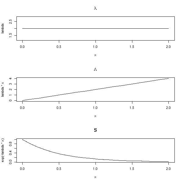
It corresponds to a constant hazard function.
lambda(t) = lambda
Lambda(t) = lambda t
S(t) = exp( - lambda t )

op <- par(mfrow=c(3,1))
n <- 20
lambda <- rep(2,n)
x <- seq(0,2,length=n)
plot(lambda ~ x, type='l', main=expression(lambda))
plot(lambda*x ~ x, type='l', main=expression(Lambda))
plot(exp(-lambda*x) ~ x, type='l', main="S")
par(op)
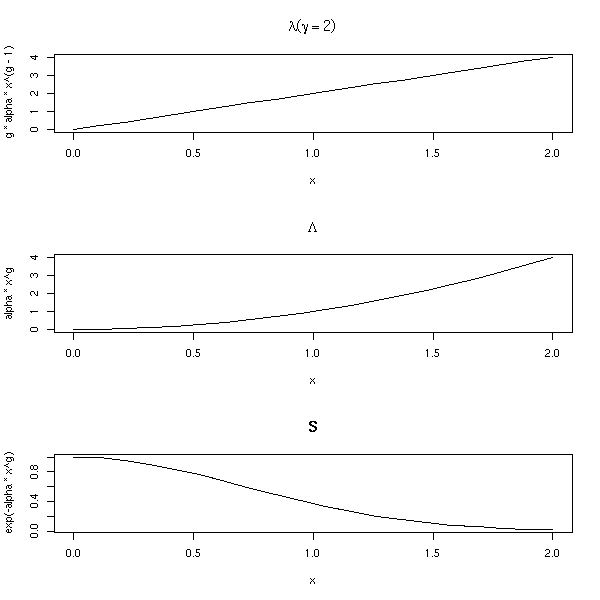
It corresponds to a hazard function of the form
Lambda(t) = a * t ^ gamma
S(t) = exp( - a * t ^ gamma )

op <- par(mfrow=c(3,1))
n <- 20
alpha <- 1
g <- rep(2,n)
x <- seq(0,2,length=n)
plot(g * alpha * x^(g-1) ~ x, type='l', main=expression(lambda (gamma==2)))
plot(alpha * x^g ~ x, type='l', main=expression(Lambda))
plot(exp(-alpha*x^g) ~ x, type='l', main="S")
par(op)
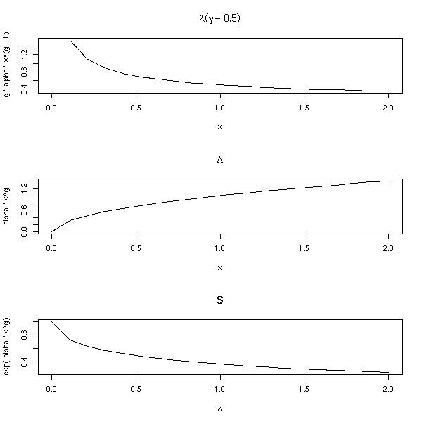
op <- par(mfrow=c(3,1))
n <- 20
alpha <- 1
g <- rep(.5,n)
x <- seq(0,2,length=n)
plot(g * alpha * x^(g-1) ~ x, type='l', main=expression(lambda (gamma==.5)))
plot(alpha * x^g ~ x, type='l', main=expression(Lambda))
plot(exp(-alpha*x^g) ~ x, type='l', main="S")
par(op)
This can be used, for instance, to model the time a machine works without breaking: the older the machine, the more likely it is to break down; the risk it breaks (the hazard rate) depends on its age.
Consider a very reliable machine: it is redundant, it is equivalent to three machines. For it to really break down, we have to wait until the three copies really break down.
TODO: Gamma distribution
TODO: explain
op <- par(mfrow=c(3,1))
n <- 200
x <- seq(0,5,length=n)
plot(1-plnorm(x) ~ x, type='l', main="S")
L <- function (x) { -log(1-plnorm(x)) }
plot(L(x) ~ x, type='l', main=expression(Lambda))
h <- .001
plot( (L(x+h)-L(x))/h ~ x, type='l', main=expression(lambda))
par(op)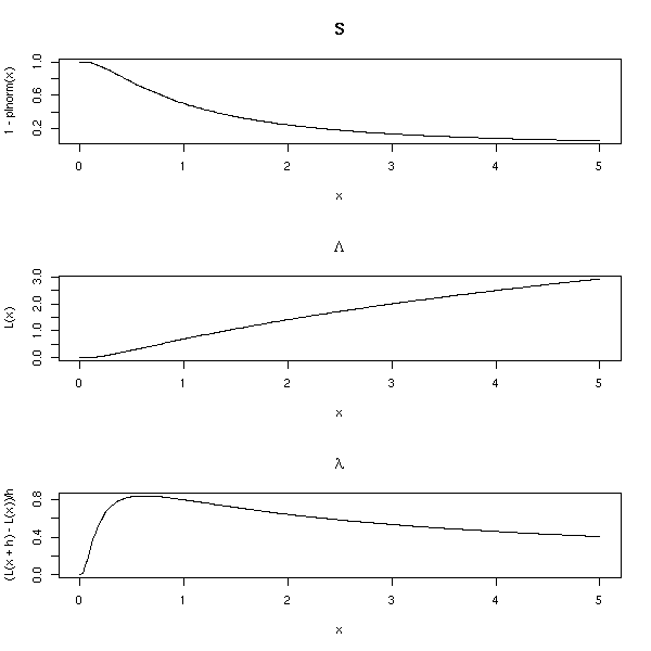
Weibul: lambda = alpha * t^(alpha-1) * exp(+X beta)
???
TODO: there is a predictive variable, it does not belong here (yet)

log-logistic model:

                  1
S(t) = --------------------------  with lambda = exp(- X beta)
        1 + (lambda t)^(1/gamma)


Gompertz: lambda = exp( exp(+X beta) + gamma t )
(important)

Generalized Gamma
(generalizes the preceding models: kappa=1:Weibul,
kappa=0:lognormal, kappa=sigma:gamma)
There are also discrete-time models:
logistic
complementary log-log
If there is no censorship, we can estimate the survival function as:
        Card( i : T_i>t )
S(t) = -------------------
              n
If there are censored data, we take them into account until their value, and then, we forget them. More precisely, it the time is discrete,
S(t0) = P(alive at t=t0 | alive at t=t0-1) * P(alive at t=t0-1)
For instance, the survival function of
1 2 2 2+ 3+ 3+ 3+ 4 4 4 4 ... (100 subjects)
can be computed as follows:
time subjects  dead censored       p1     p2    S=p1*p2
-------------------------------------------------------
1         100     1        0   99/100      1        .99
2          99     2        1   97/100    .99      .9603
3          96     0        3   96/100  .9603      .9219
4          93     3        0   90/100  .9219      .8297
The values of S are the products:
S(0) = 1
S(1) = 1 * 99/100
S(2) = 1 * 99/100 * 97/100
S(3) = 1 * 99/100 * 97/100 * 96/100
S(4) = 1 * 99/100 * 97/100 * 96/100 * 90/100
etc.
We can give a general formula:
                                di
S(t) =      Product      ( 1 - ---- )
       i such that ti<t         ni
We can compute confidence intervals if we assume that Lambda (i.e., -log(S)) is approxsimately gaussian.
TODO
PROBLEM: Where do we get the variance of Lambda from?
There are other estimators of the survival function, for instance the Altschuler--Nelson--Aalen--Flemming--Harrington one:
                               di
Lambda(t) =        Sum       ------.
            i such that ti<t   ni
Those estimators have a high variance: if you have a reasonnable model, prefer a Maximum Likelihood parametric estimator (actually, the Kaplan--Meier estimator is a "maximum likelihood non parametric estimator").
Most of the functions are in the "survival" package.
The "Surv" functions creates survival variables.
> Surv(c(1,2,2,2,3,3,3,4,4,4,4),
+      c(1,1,1,0,0,0,0,1,1,1,1))
[1] 1  2  2  2+ 3+ 3+ 3+ 4  4  4  4
The "survfit" computes the survival function
> x <- Surv(c(1,2,2,2,3,3,3,4,4,4,4),
+           c(1,1,1,0,0,0,0,1,1,1,1))

> survfit(x)
Call: survfit(formula = x)
        n    events     rmean se(rmean)    median   0.95LCL   0.95UCL
   11.000     7.000     3.364     0.322     4.000       Inf       Inf

> summary(survfit(x))
Call: survfit(formula = x)
 time n.risk n.event survival std.err lower 95% CI upper 95% CI
    1     11       1    0.909  0.0867        0.754            1
    2     10       2    0.727  0.1343        0.506            1
    4      4       4    0.000      NA           NA           NA
that can then be plotted.
set.seed(87638)
library(survival)
# survfit <- survival:::survfit # Incompatibility Design/survival?
try( detach("package:Design") )
n <- 200
x <- rweibull(n,.5)
y <- rexp(n,1/mean(x))
s <- Surv(ifelse(x<y,x,y), x<=y)
plot(s) # not insightful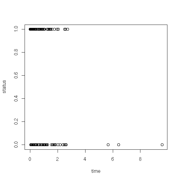
plot(survfit(s))
lines(survfit(s, type='fleming-harrington'), col='red')
r <- survfit(s)
lines( 1-pweibull( r$time, .5 ) ~ r$time, lty=3, lwd=3, col='blue' )
legend( par("usr")[2], par("usr")[4], yjust=1, xjust=1,
        c("Kaplan-Meier", "Fleming-Harrington", "Theoretical survival function"),
        lwd=c(1,1,3), lty=c(1,1,3),
        col=c(par("fg"), 'red', 'blue'))
title(main="Survival function (Kaplan-Meier estimator)")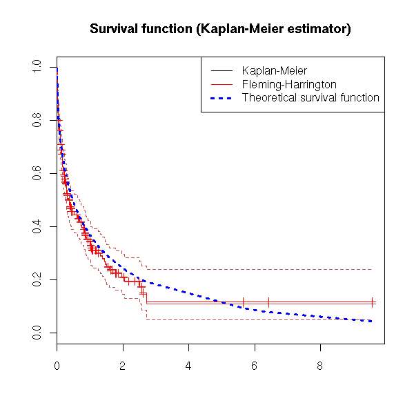
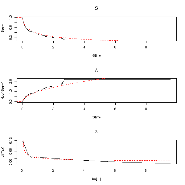
op <- par(mfrow=c(3,1))
r <- survfit(s)
plot(r$surv ~ r$time, type='l', main="S")
curve( 1-pweibull(x,.5,1), col='red', lty=2, add=T )
plot(-log(r$surv) ~ r$time, type='l', main=expression(Lambda))
curve( -log(1-pweibull(x,.5,1)), col='red', lty=2, add=T )
# Before derivating, we smooth Lambda
a <- -log(r$surv)
b <- r$time
# library(modreg) # Merged into stats...
l <- loess(a~b)
bb <- seq(min(b),max(b),length=200)
aa <- predict(l, data.frame(b=bb))
plot( diff(aa) ~ bb[-1], type='l', main=expression(lambda) )
aa <- -log(1-pweibull(bb,.5,1))
lines( diff(aa) ~ bb[-1], col='red', lty=2 )
par(op)
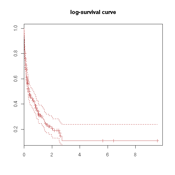
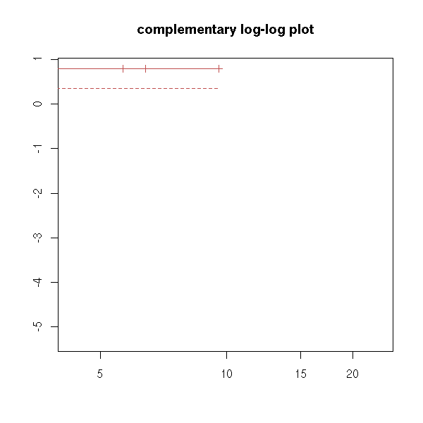
Actually, you can get some of those plots using the "fun" argument of the "plot.survfit" function.
plot(r, fun="log", main="log-survival curve")
plot(r, fun="event", main="cumulative events: f(y)=1-y")
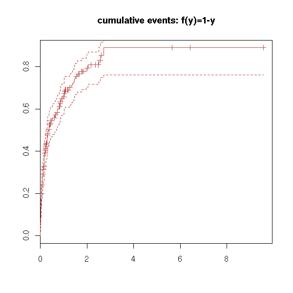
plot(r, fun="cumhaz", main="cumulative hazard: f(y)=-log(y)=Lambda")
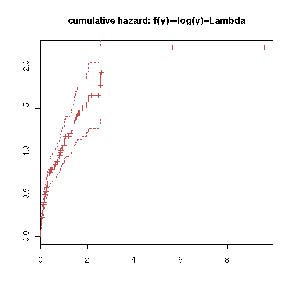
try(
  plot(r, fun="cloglog", main="complementary log-log plot")
)
# f(y)=log(-log(y)), log-scale on the x-axis
You can also have one (or several) qualitative predictive variables -- more about this later -- hopefully.
n <- 200
x1 <- rweibull(n,.5)
x2 <- rweibull(n,1.2)
f <- factor( sample(1:2, n, replace=T), levels=1:2 )
x <- ifelse(f==1,x1,x2)
y <- rexp(n,1/mean(x))
s <- Surv(ifelse(x<y,x,y), x<=y)
plot(s, col=as.numeric(f))
plot( density(s[,1][ s[,2] == 1 & f == 1]), lwd=3,
      main="Survival analysis, one factor" )
lines( density(s[,1][ s[,2] == 0 & f == 1]), lty=2, lwd=3 )
lines( density(s[,1][ s[,2] == 1 & f == 2]), col='red', lwd=3 )
lines( density(s[,1][ s[,2] == 0 & f == 2]), lty=2, col='red', lwd=3 )
legend( par("usr")[2], par("usr")[4], yjust=1, xjust=1,
        c("non censored, f = 1", "censored, f = 1",
          "non censored, f = 2", "censored, f = 2"),
        lty=c(1,2,1,2),
        lwd=1,
        col=c(par('fg'), par('fg'), 'red', 'red') )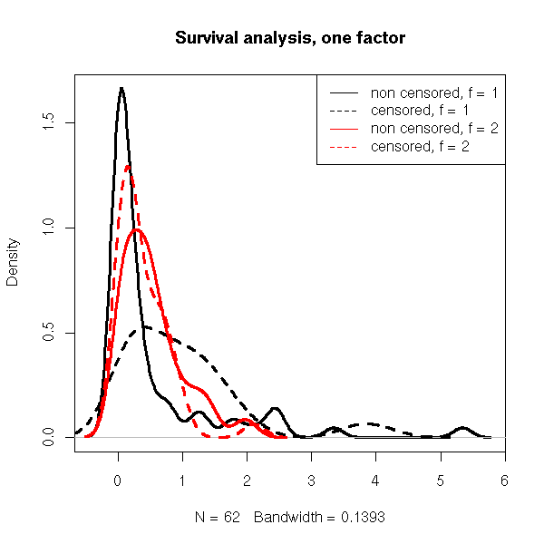
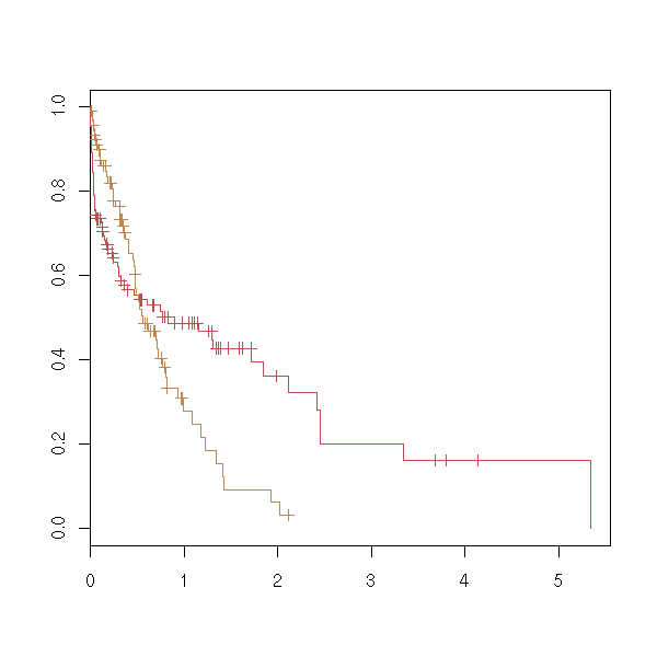
plot(survfit(s ~ f), col=as.numeric(levels(f)))
TODO: with two qualitative predictive variables.
survfit(s~f1+f2)
TODO: and what if is not a factor? (later, when we perform regressions).
TODO: Choose two examples, one with predictive variables, one without, with which we will play until the end of the chapter.
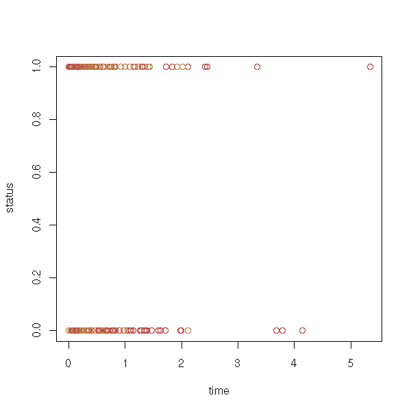
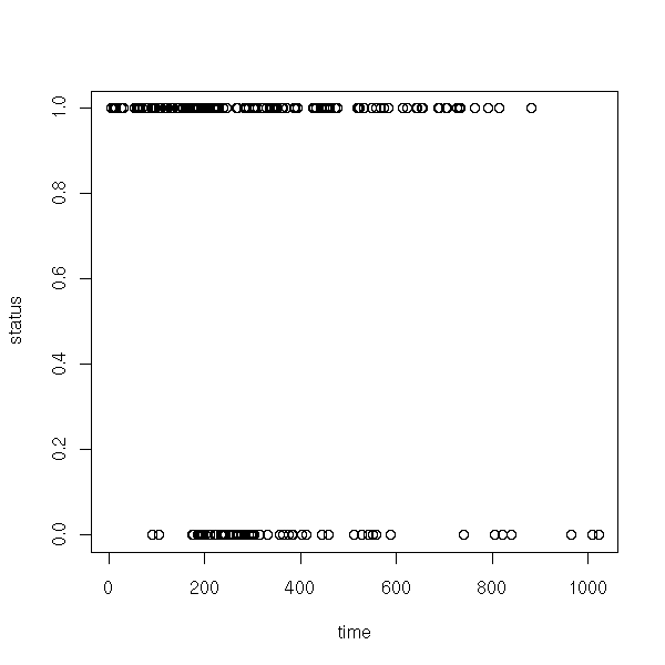
data(lung)
x <- Surv(lung$time, lung$status)
plot(x)
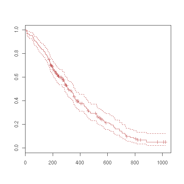
plot(survfit(x))
We can wonder if a survival variable depends on a factor.
data(lung)
y <- Surv(lung$time, lung$status)
x <- lung$sex
summary(coxph(y~x))

Rsquare= 0.046   (max possible= 0.999 )
Likelihood ratio test= 10.6  on 1 df,   p=0.00111
Wald test            = 10.1  on 1 df,   p=0.00149
Score (logrank) test = 10.3  on 1 df,   p=0.00131
TODO

Discrete hazard rate:
h(aj) = P[  a(j-1) < T <= a(j) | T > a(j-1)  ]
TODO: write the survival function as a function of h.

TODO:
LifeTable: This is the discrete equivalent of the Kaplan-Meier estimator.
TODO: Introduction
We are now about to add predictive variables.

Some do not depend on the subject (but depend on time):
inflation, unemployment rate, mean temperature in summer, etc.

Others depend on the subject and may depend on time (SES, age, blood
preasure) or not (sex).

Methods:
- parametric
- semi-parametrix (Cox regression): parametric for the part that
  depends on the predictiva variables, non-parametric (Kaplan-Meier)
  for the rest.
TODO: Classification of the various models.
Continuous:
  Exponential (PH and AFT)
  Weibull (PH and AFT)
  Gompertz (PH)
  lognormal (AFT)
  loglogistic (AFT)
  generalized gamma (AFT)

discrete:
  logistic (proportionnal odds)
  cloglog (PH)

PH (Proportionnal Hazards): lambda = lambda0(t) * exp(X beta)

AFT (Accelerated Failure Time): T = exp(-X beta) * exp(z)
TODO: the "survreg" function???
We can first do the computations by hand, by explicitely writing the log-likelihood.
Prod( f(b,x_i) where i is not censored ) * Prod( S(b,x_i) where i is censored )
You can object that there should be a factor for the probability of censorship: we shall assume it is independant of the outcome of the experiment and forget it.
You can maximize the log-likelihood with the "optim" function -- but be careful with the choice of the initial parameters.
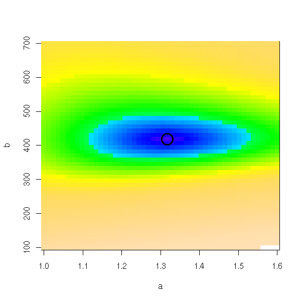
To check that it is indeed a minimum, we can plot the log-likelohood (here, we only have two parameters to estimate: it there was a simgle parameter, we would draw the curve of the log-likelihood; if there were more, it would be more troublesome to plot -- with just three variables, we could use an animation or a treillis plot).
data(lung)
x <- Surv(lung$time, lung$status)
f <- function (p,t) { dweibull(t,p[1],p[2]) }
S <- function (p,t) { 1-pweibull(t,p[1],p[2]) }
ll <- function (p) {
  time <- x[,1]
  status <- x[,2]
  censored <- 0
  dead <- 1
  # cat(p); cat("\n"); str(time); cat("\n");
  -2*( sum(log(f(p,time[status==dead]))) + sum(log(S(p,time[status==censored]))) )
}

# Estimations of the second parameter
m <- 1     # Does not work
m <- 100
s <- survfit(x)
m <- mean(s$time)
m <- max(s$time[s$surv>.5])

r <- optim( c(1,m), ll )

# Plot the log-likelohood
myOuter <- function (x,y,f) {
  r <- matrix(nrow=length(x), ncol=length(y))
  for (i in 1:length(x)) {
    for (j in 1:length(y)) {
      r[i,j] <- f(x[i],y[j])
    }
  }
  r
}
lll <- function (u,v) {
  r <- ll(c(u,v))
  if(r==Inf) r <- NA
  r
}
a <- seq(1,1.6,length=50)
b <- seq(100,700,length=50)
ab <- myOuter(a,b,lll)
persp(a,b,ab)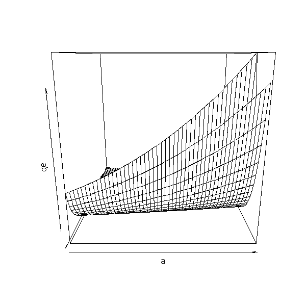
op <- par(mfrow=c(3,3))
for (i in seq(0,360,length=10)[-10]) {
  persp(a,b,ab,theta=i)
}
par(op)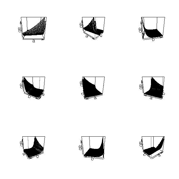
We could also use xgobi:
xgobi(data.frame(
  x=rep(a,1,each=length(b)),
  y=rep(b,length(a)),
  z=as.vector(ab))
)
But it is probably clearer in dimension 2:
image(a,b,ab)
points(r$par[1],r$par[2],lwd=3,cex=3)
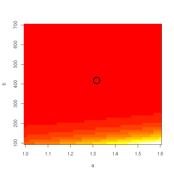
With the default colors, we do not see anything.
n <- 255
image(a,b,ab, col=topo.colors(n), breaks=quantile(ab,(0:n)/n, na.rm=T))
points(r$par[1],r$par[2],lwd=3,cex=3)
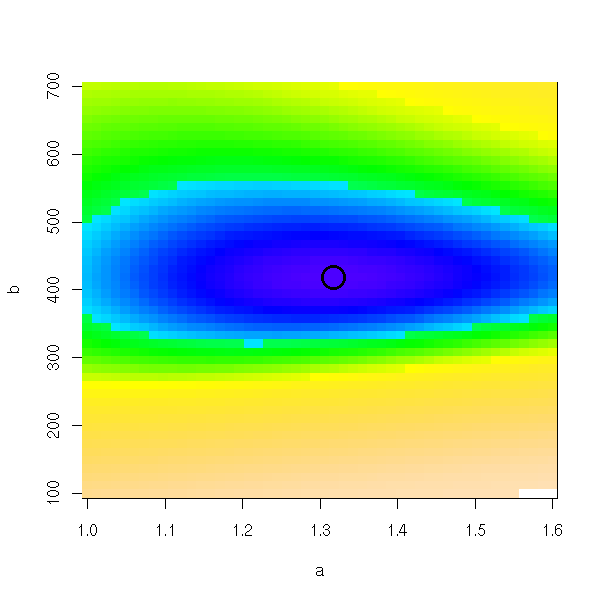
Or even, to stress the differences around the minimum:
image(a,b,ab, col=topo.colors(n), breaks=quantile(ab,((0:n)/n)^2,na.rm=T))
points(r$par[1],r$par[2],lwd=3,cex=3)
We could do the same king of plots with the "lattice" library.
A FAIRE
library(lattice)
?levelplot
?contourplot
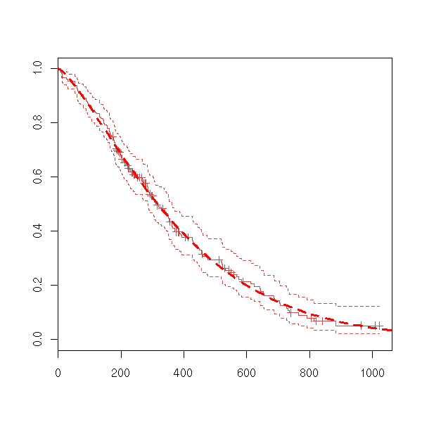
You can compare the Kaplan-Meier curve with the theoretical one:
plot(survfit(x))
curve( 1-pweibull(x,r$par[1],r$par[2]), add=T, col='red', lwd=3, lty=2 )
Let us take an example and try to model it with an exponential model, a Weibull model and a Gamma model.
ph.mle.weibull <- function (x) {
  f <- function (p,t) { dweibull(t,p[1],p[2]) }
  S <- function (p,t) { 1-pweibull(t,p[1],p[2]) }
  m <- mean(survfit(x)$time)
  ph.mle.optim(x,f,S,c(1,m))
}
ph.mle.exp <- function (x) {
  f <- function (p,t) { dexp(t,p) }
  S <- function (p,t) { 1-pexp(t,p) }
  m <- mean(survfit(x)$time)
  ph.mle.optim(x,f,S,1/m)
}
ph.mle.gamma <- function (x) {
  f <- function (p,t) { dgamma(t,p[1],p[2]) }
  S <- function (p,t) { 1-pgamma(t,p[1],p[2]) }
  m <- mean(survfit(x)$time)
  ph.mle.optim(x,f,S,c(1,1/m))
}
ph.mle.optim <- function (x,f,S,m) {
  ll <- function (p) {
    time <- x[,1]
    status <- x[,2]
    censored <- 0
    dead <- 1
    -2*( sum(log(f(p,time[status==dead]))) + sum(log(S(p,time[status==censored]))) )
  }
  optim(m,ll)
}
eda.surv <- function (x) {
  r <- survfit(x)
  plot(r)
  a1 <- ph.mle.exp(x)$par
  lines( 1-pexp(r$time,a1) ~ r$time, col='red' )
  a2 <- ph.mle.weibull(x)$par
  lines( 1-pweibull(r$time,a2[1],a2[2]) ~ r$time, col='green' )
  a3 <- ph.mle.gamma(x)$par
  lines( 1-pgamma(r$time,a3[1],a3[2]) ~ r$time, col='blue' )
  legend( par("usr")[2], par("usr")[4], yjust=1, xjust=1,
          c(paste("Exponential(", signif(a1,2), ")", sep=''),
            paste("Weibull(", signif(a2[1],2), ", ", signif(a2[2],2), ")", sep=''),
            paste("Gamma(", signif(a3[1],2), ", ", signif(a3[2],2), ")", sep='')
          ),
          lwd=1, lty=1,
          col=c('red', 'green', 'blue'))
  title(main="Parametric estimation of PH models")
}

data(lung)
x <- Surv(lung$time, lung$status)
eda.surv(x)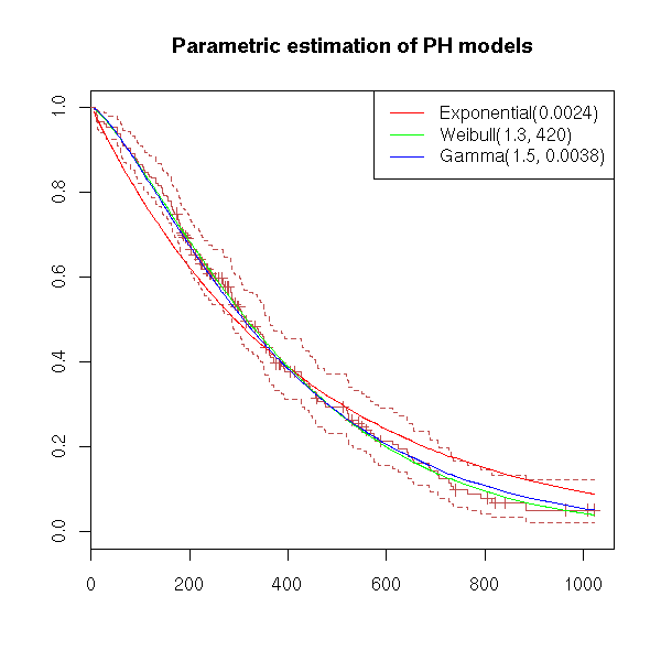
To assess the quality of the estimation, we can use a quantile-quantile plot.
x <- Surv(lung$time, lung$status)
r <- survfit(x)
a1 <- ph.mle.exp(x)$par
t1 = 1-pexp(r$time,a1)
a2 <- ph.mle.weibull(x)$par
t2 <- 1-pweibull(r$time,a2[1],a2[2])
a3 <- ph.mle.gamma(x)$par
t3 <- 1-pgamma(r$time,a3[1],a3[2])
plot( t1 ~ r$surv, col='red', xlab='sample', ylab='model')
points( t2 ~ r$surv, col='green')
points( t3 ~ r$surv, col='blue' )
abline(0,1)
legend( par("usr")[1], par("usr")[4], yjust=1, xjust=0,
        c(paste("Exponental(", signif(a1,2), ")", sep=''),
          paste("Weibull(", signif(a2[1],2), ", ", signif(a2[2],2), ")", sep=''),
          paste("Gamma(", signif(a3[1],2), ", ", signif(a3[2],2), ")", sep='')
        ),
        lwd=1, lty=1,
        col=c('red', 'green', 'blue'))
title(main="Parametric estimation of PH models")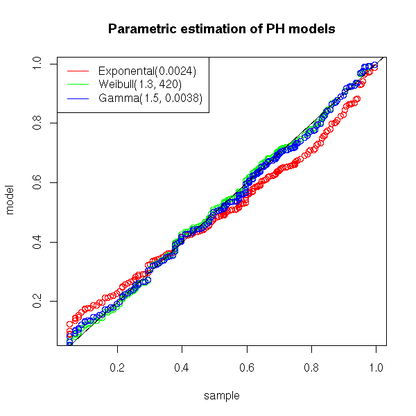
We can also plot the residuals (the difference between the non parametric (Kaplan-Meier) estimation and the parametric estimation of the survival function.
plot( t1 - r$surv ~ t1, col='red', xlab='predicted values', ylab='residuals')
points( t2 - r$surv ~ t2, col='green')
points( t3 - r$surv ~ t3, col='blue' )
abline(h=0, lty=3)
legend( par("usr")[2], par("usr")[4], yjust=1, xjust=1,
        c(paste("Exponential(", signif(a1,2), ")", sep=''),
          paste("Weibull(", signif(a2[1],2), ", ", signif(a2[2],2), ")", sep=''),
          paste("Gamma(", signif(a3[1],2), ", ", signif(a3[2],2), ")", sep='')
        ),
        lwd=1, lty=1,
        col=c('red', 'green', 'blue'))
title(main="Parametric estimation of PH models")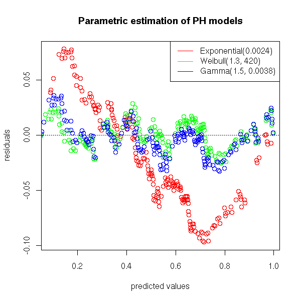
plot( abs(t1 - r$surv) ~ t1, col='red',
      xlab='predicted values', ylab=expression( abs(residuals) ))
points( abs(t2 - r$surv) ~ t2, col='green')
points( abs(t3 - r$surv) ~ t3, col='blue' )
abline(h=0, lty=3)
legend( par("usr")[2], par("usr")[4], yjust=1, xjust=1,
        c(paste("Exponental(", signif(a1,2), ")", sep=''),
          paste("Weibull(", signif(a2[1],2), ", ", signif(a2[2],2), ")", sep=''),
          paste("Gamma(", signif(a3[1],2), ", ", signif(a3[2],2), ")", sep='')
        ),
        lwd=1, lty=1,
        col=c('red', 'green', 'blue'))
title(main="Parametric estimation of PH models")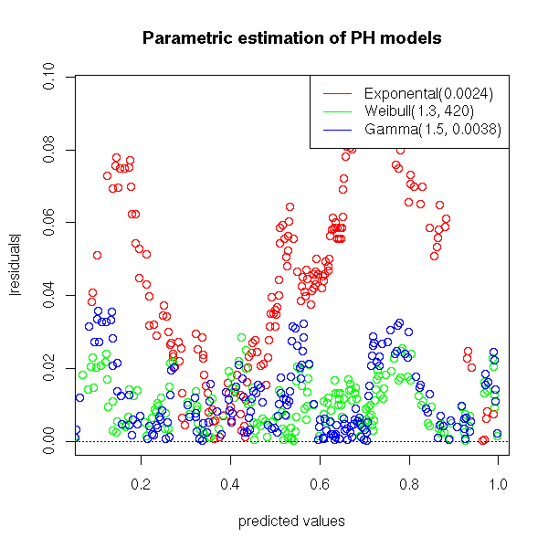
TODO: Add a test to check if, under a Weibull model, the
data are very different from an exponential one (i.e.,
test if the first parameter is really different from one).
Put this test in "eda.surv" and add the result to the
plot.
If we get back to our simulated example (Weibull, parameters .5 and 1), we get values close to the theoretical ones.
> n <- 200
> x <- rweibull(n,.5)
> y <- rexp(n,1/mean(x))
> s <- Surv(ifelse(x<y,x,y), x<=y)
> ph.mle.weibull(s)$par
[1] 0.4891810 0.9924432
TODO: tests...
TODO: diagnostic plots...
If you want to predict a survival variable from another variable X, you can try the following model
lambda(t|X) = lambda(t) * exp(X*b)
where lambda is an underlying hazard function (corresponding, say, to a Weibull model) and b is a parameter to be estimated. To find b and the parameters of the underlying model, we still us the Maximum Likelihood method.
TODO: example

data(lung)
y <- Surv(lung$time, lung$status)
x1 <- lung$age
x2 <- lung$meal.cal


TODO: Add b in the following code...
I cannot get a simple and general expression of the log-likelihood
(I have an integral of lambda that appears...)

f <- function (p,t) { dweibull(t,p[1],p[2]) }
S <- function (p,t) { 1-pweibull(t,p[1],p[2]) }
m <- mean(survfit(y)$time)
ll <- function (p) {
  time <- y[,1]
  status <- y[,2]
  censored <- 0
  dead <- 1
  -2*( sum(log(f(p,time[status==dead]))) + sum(log(S(p,time[status==censored]))) )
}
optim(m,ll)
Actually, the "survreg" function already provides us with that result.
TODO: understand
Exokain why it is the same result.

> summary(survreg(y~x1+x2))
Call:
survreg(formula = y ~ x1 + x2)
                Value Std. Error      z        p
(Intercept)  6.82e+00    0.57891 11.785 4.64e-32
x1          -1.35e-02    0.00809 -1.667 9.55e-02
x2           2.37e-05    0.00018  0.131 8.95e-01
Log(scale)  -2.54e-01    0.06973 -3.641 2.71e-04
Scale= 0.776
Weibull distribution
Loglik(model)= -930.6   Loglik(intercept only)= -932.2
        Chisq= 3.17 on 2 degrees of freedom, p= 0.21
Number of Newton-Raphson Iterations: 4
n=181 (47 observations deleted due to missing)

TODO: To check that I have correctly understood the result,
do a simulation (Weibul, parameters .5 and 3, b=c(1 2 -1)) and give
it to "survreg".

TODO: an example with predictive variables that do not
depend on time TODO: an example with predictive variables
that depend on time.
We assume that the survival variable T is given by
ln(T) = beta X + error
where the error term follows a certain distribution (for instance, if it is a gaussian distribution, T is log-normal).
TODO: extreme value distribution with 2 parameters (this yields
the Weibul distribution)
You can also write those models:
ln(psi * T) = error
psi = exp(-beta X)
Note that psidoes not depend on T; furthermore, if psi>1, they die more quickly, if psi<1, they die more slowly -- hence the name "Accelerated Failure Time".
These are simply gemeralized linear models
TODO
?glm
This is a PH model in which lambda (the underlying Hazard function) is pievewise constant -- the experimentor chooses the times at which the value changes.
This is a first analysis, a bit simplistic, of what can be done when the predictors depend on time.
TODO: an example
In a "Proportional Hazard Model",
lambda = lambda0 * exp(b * X)
you can actually estimate the coefficients b of the regression, without taking lambda0 into account, with a partial likelihood.
TODO: Where does this "partial likelihood" come from?
library(survival)
?survfit
?survreg
?coxph

Proportionnal hazard:  lambda(t|X) = lambda(t) exp(X beta)

Cox proportional hazard model
A popular semi-parametric model for survival analysis -- as efficient as parametric models,
even when those apply.
The model is still lambda(t|X) = lambda(t) exp(X beta), but we do not assign a prescribed form to lambda.

Predictive variables: they can depend on time -- it really
complicates things.
See the ICE package.
There can be several events in the series, for instance, several kinds of death, or a final event (death) preceded by several non lethal events (heart attack, high blood pressure diagnosis, surgery, etc.)
TODO: example
If there are two independant lethal events, they can be tackled
separately.
  Violent death:          1 1 1 3
  Disease-related death:  1 2 4 5 5 6
  Alive:                  7+ 7+ 7+
To study violent deaths:
  1  1  1  3  1+ 2+ 4+ 5+ 5+ 6+ 7+ 7+ 7+
To study disease-related deaths:
  1+ 1+ 1+ 3+ 1  2  4  5  5  6  7+ 7+ 7+

If the events are not independant (for instance, death by
cancer and by heart attack can have a common cause:
tobacco), the results would be biased.
We can also imagine the following situation: all the patients have a hazard function of the same form, up to a multiplicative factor. If we had enough predictive variables, we would try to predict this factor, but if we have none (or not enough), we cannot reliably predict it. In that case, we can consider a model of the form
lambda(t) = lambda0(t) * u
where u is a random variable, positive, with mean 1. As the value of u changes from one subject to the next, we will not be able to predict it, but, at least, we can predict its variance.
TODO: How do we do this?

TODO: in R?

frail.fit(eha)          Fits a frailty proportional hazards model
frailty(survival)       (Approximate) Frailty models
mlefrailty.fit(survrec)
                        Survival function estimator for correlated
                        recurrence time data under a Gamma Frailty
                        Model
Recurrent failure times
library(survrec)

Penalized maximum likelihood
?pspline
?frailty
?ridge

The Kaplan-Meier curves should not cross: it indicates that
the PH model does NOT hold.

You can use survival analysis even when the observations are not
censored: the notions (hazard function, etc.) and the plots may be
relevant.
A few packages allow us to manipulate spacial data:
geoR (see rather geoRglm)
geoRglm
spatstat
fields
grasper
pastecs
spatial
splancs
GRASS (devel)
gstat
For more details, see for example:
http://freegis.org/index.en.html

TODO
http://www.sasi.group.shef.ac.uk/worldmapper/
http://aps.arxiv.org/abs/physics/0401102/
Plotting a spacial process (this could actually be any 2-dimensional process, regardless of the interpretation of those two dimensions) does not always give enough insight. To improve this plot, one can "decorate" it with various graphs. The most useful is probably the minimum spanning tree (MST): if there is a functional relation between the two variables, or of the points tend to lie on a 1-dimensional subspace, this will become obvious -- even more so if you consider a pruned MST.
Other potentiall useful decorations include: a minimum length path (this is the traveling salesman problem (TSP)), the nearest neighbour graph (each point is connected to the closest -- this is actually a subgraph of the MST), the convex hull, the alpha hull, the Voronoi mosaic, the Delaunay triangulation, etc.
x <- runif(100)
y <- runif(100)
nearest_neighbour <- function (x, y, d=dist(cbind(x,y)), ...) {
  n <- length(x)
  stopifnot(length(x) == length(y))
  d <- as.matrix(d)
  stopifnot( dim(d)[1] == dim(d)[2] )
  stopifnot( length(x) == dim(d)[1] )
  i <- 1:n
  j <- apply(d, 2, function (a) order(a)[2])
  segments(x[i], y[i], x[j], y[j], ...)
}
plot(x, y,
     main="Nearest neighbour graph",
     xlab = "", ylab = "")
nearest_neighbour(x, y)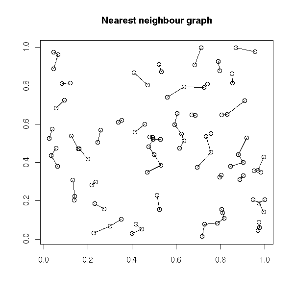
plot(x, y,
     main = "Minimum spanning tree",
     xlab = "", ylab = "")
nearest_neighbour(x, y, lwd=10, col="grey")
points(x,y)
library(ape)
r <- mst(dist(cbind(x, y)))
i <- which(r==1, arr.ind=TRUE )
segments(x[i[,1]], y[i[,1]], x[i[,2]], y[i[,2]],
         lwd = 2, col = "blue")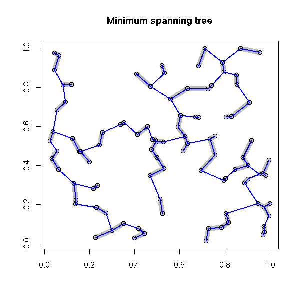
# Voronoi diagram
library(tripack)
plot(voronoi.mosaic(x, y))
segments(x[i[,1]], y[i[,1]], x[i[,2]], y[i[,2]],
         lwd=3, col="grey")
points(x, y, pch=3, cex=2, lwd=3)
box()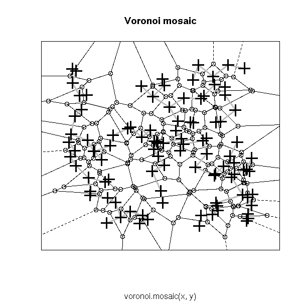
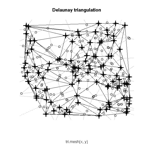
# Delaunay triangulation
# See also the "deldir" package
plot(tri.mesh(x,y))
plot(voronoi.mosaic(x, y), add=T, col="grey")
points(x, y, pch=3, cex=2, lwd=3)
http://cfa-www.harvard.edu/~huchra/zcat/

wget http://cfa-www.harvard.edu/~huchra/zcat/n36.dat
The file looks like
1234567890X12121234X1212123456123456
Name        RA (1950) Dec Mag   Vh  sig sour type  D1 D2  BT    UGC      RFN    Comments and other names
08003+3336 080018.0 33360014.7 1173515010510 1  P                               AK151
08005+3529 080030.0 35290015.4 10079 441-1  -1                           T11956
N2649      084059.1 34535613.1  4235 2010617 4X2R 1.7 1.6      04555
08410+3342 084100.8 33415015.2  7656 301-1   4A / 1.8 0.3      04558     T12403
08422+3437 084212.0 34370014.7  7691 311-1   1B P                        T12067
08424+3707 084224.0 37070013.8  392315010510 0    0.7 0.7      04572            MK626,M6-19-21,AK176
It is a fixed-width file, that can be read as
w <- c(
  name = 10,
  -1,
  ra.hour = 2,
  ra.min  = 2,
  ra.sec  = 4,
  -1,
  dec.deg = 2,
  dec.min = 2,
  dec.sec = 6)
  v.helio = 7,
  v.err = 3,
  b.source = 1,
  v.source = 2,
  v.source2 = 2,
  t.type = 2,
  bar.type = 1,
  lum.class = 1,
  struct = 1,
  d1.min = 4,
  d2.min = 2,
  bt.mag = 6,
  ugc = 6,
  d.mpc = 4,
  space = 1,
  ra.hr.1950 = 2,
  ra.min.1950 = 2,
  ra.sec.1950 = 5,
  dec.sign.1950 = 1,
  dec.deg.1950 = 2,
  dec.min.1950 = 2,
  dec.sec.1950 = 4,
  space = 1,
  rfn = 6,
  flag = 1,
  comments = 78
)

x <- read.fwf("/tmp/n36.dat", w,
              skip = 31,
              nrows = 718,
              col.names = names(w) [ names(w) != "" ],
              row.names = NULL)
y <- x
y$dec.sec <- as.numeric(as.character(y$dec.sec))
y$ra  <- y$ra.hour +  y$ra.min/60 +  y$ra.sec/3600
y$dec <- y$dec.deg + y$dec.min/60 + y$dec.sec/3600
y <- y[,c("ra", "dec")]
plot(y)
Other applications:
mesh generation (with centroidal vorinoi tessellation, i.e., Voronoi
tessallations, i.e., the center of each tile is its center of
gravity) to solve PDE.
One can compute a centroidal Voronoi tessallation as follows: take a set of points, compute their Voronoi tessallation, replace the points by the center of gravity of their tiles, iterate until convergence.
TODO: Implement this

library(tripack)
set.seed(1)
n <- 20
x <- runif(n)
y <- runif(n)
v <- voronoi.mosaic(x, y)
plot(v, main="Voronoi mosaic and tile centers")
points(x,y, pch=3, cex=1.5, lwd=2)

# Center of gravity of a convex polygon, given by
# the coordinates of its vertices.
voronoi.center <- function (x,y) {
  stopifnot( length(x) == length(y) )
  n <- length(x)
  # A point inside the polygon
  x0 <- mean(x)
  y0 <- mean(y)
  # Reorder the vertices
  o <- order(atan2(y-y0, x-x0))
  x <- x[o]
  y <- y[o]
  # Duplicate the first point at the end, for the loop
  x <- c(x, x[1])
  y <- c(y, x[1])
  # Compute the center of gravity and the area of each triangle
  gx <- gy <- rep(NA, n)
  a <- rep(NA, n)
  for (i in 1:n) {
    xx <- c( x0, x[i], x[i+1] )
    yy <- c( y0, y[i], y[i+1] )
    gx[i] <- mean(xx)
    gy[i] <- mean(yy)
    a[i] <- voronoi.polyarea(xx, yy)
  }
  # Compute the barycenter of those centers of gravity, with
  # weights proportionnal to the triangle areas.
  res <- c(
     x = weighted.mean(gx, w=a),
     y = weighted.mean(gy, w=a)
   )
   attr(res, "x") <- x[1:n]
   attr(res, "y") <- y[1:n]
   attr(res, "G") <- c(x0,y0)
   attr(res, "gx") <- gx
   attr(res, "gy") <- gy
   res
}
voronoi.centers <- function (v) {
  ntiles <- length(v$tri$x)
  res <- matrix(NA, nc=2, nr=ntiles)
  for (i in 1:ntiles) {
    vs <- voronoi.findvertices(i, v)
    if (length(vs) > 0) {
      res[i,] <- voronoi.center(v$x[vs], v$y[vs])
    }
    else {
      res[i,] <- NA
    }
  }
  res
}

points( voronoi.centers(v), pch=16, col="red")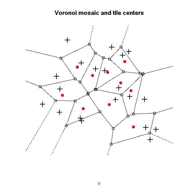
# Test of the "voronoi.center" function
k <- 5
theta <- seq(0, length=k, by=2*pi/k)
X <- rlnorm(k) * cbind(cos(theta), sin(theta))

plot(rbind(X,X[1,]), type="l")
segments(0,0,X[,1],X[,2], lty=3)
r <- voronoi.center(X[,1],X[,2])
G <- attr(r,"G")
points(G[1], G[2], col="red", pch=16)
segments(G[1],G[2],X[,1],X[,2], col="red")
points(attr(r,"gx"), attr(r,"gy"), col="red", pch=15)
segments(attr(r,"gx"), attr(r,"gy"), X[,1], X[,2], col="red")
segments(attr(r,"gx"),  attr(r,"gy"),
         X[c(k,1:(k-1)),1], X[c(k,1:(k-1)),2], col="dark green")
points(r[1], r[2], pch=3, col="blue", cex=3, lwd=5)

for (i in 1:10) {
  z <- voronoi.centers(v)
  x <- ifelse( is.na(z[,1]), x, z[,1] )
  y <- ifelse( is.na(z[,2]), y, z[,2] )
  v <- voronoi.mosaic(x, y)
}
plot(v, main="Centroidal Voronoi tessallation?")
points(x,y, pch=3, cex=1.5, lwd=2)
points( voronoi.centers(v), pch=16, col="red")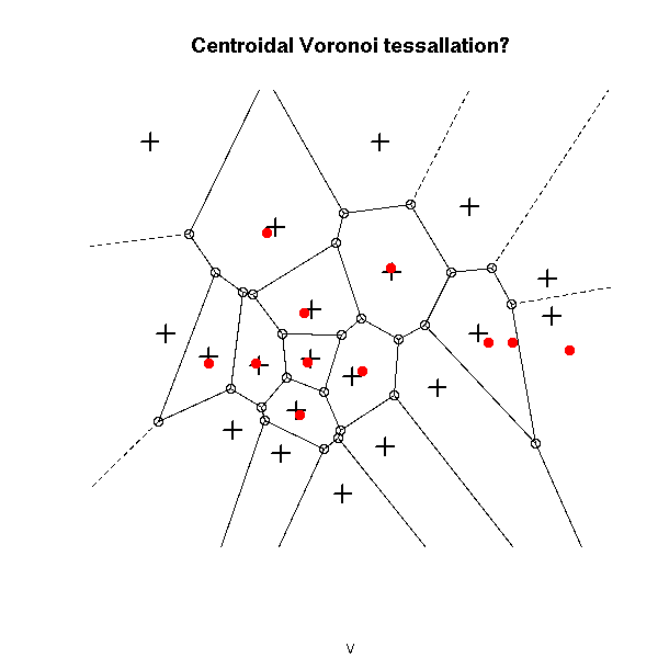
for (i in 1:10) {
  z <- voronoi.centers(v)
  x <- ifelse( is.na(z[,1]), x, z[,1] )
  y <- ifelse( is.na(z[,2]), y, z[,2] )
  v <- voronoi.mosaic(x, y)
}
plot(v, main="Centroidal Voronoi tessallation?")
points(x,y, pch=3, cex=1.5, lwd=2)
points( voronoi.centers(v), pch=16, col="red")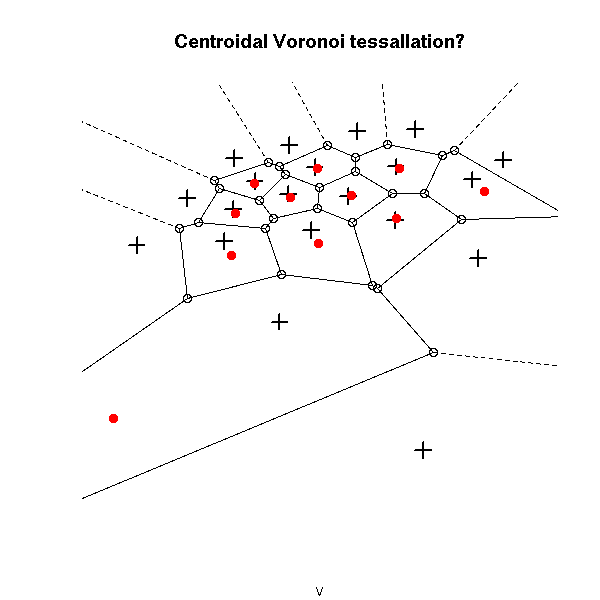
for (i in 1:10) {
  z <- voronoi.centers(v)
  x <- ifelse( is.na(z[,1]), x, z[,1] )
  y <- ifelse( is.na(z[,2]), y, z[,2] )
  v <- voronoi.mosaic(x, y)
}
plot(v, main="Centroidal Voronoi tessallation?")
points(x,y, pch=3, cex=1.5, lwd=2)
points( voronoi.centers(v), pch=16, col="red")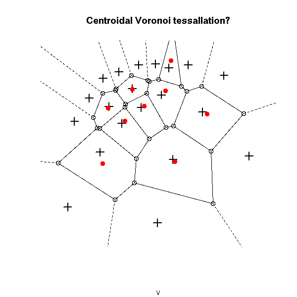
for (i in 1:10) {
  z <- voronoi.centers(v)
  x <- ifelse( is.na(z[,1]), x, z[,1] )
  y <- ifelse( is.na(z[,2]), y, z[,2] )
  v <- voronoi.mosaic(x, y)
}
plot(v, main="Centroidal Voronoi tessallation?")
points(x,y, pch=3, cex=1.5, lwd=2)
points( voronoi.centers(v), pch=16, col="red")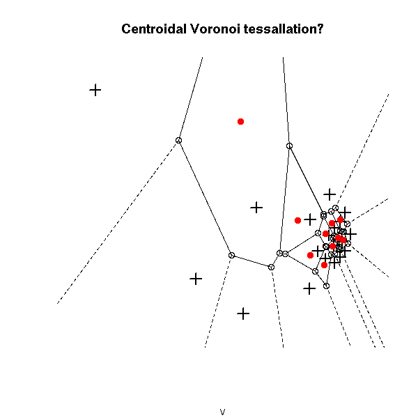
TODO:
- Check that my "voronoi.center" function works as advertised
  (I have a few doubts).
- Change the loop inside "voronoi.centers" so as to include the
  "degenerate" cells as well.
Here is another way of getting a centroidal Voronoi tessallation: take points at random, apply the k-means algorithm, compute the Voronoi diagram of the resulting centers. If there were sufficiently many points to begin with, the result will be sufficiently close to a centroidal Voronoi tessellation.
library(tripack)
n <- 100    # Number of cells
k <- 100    # Number of points in each cell
x <- runif(k*n)
y <- runif(k*n)
z <- kmeans(cbind(x,y), n)
v <- voronoi.mosaic( z$centers[,1], z$centers[,2] )
plot(v, main="Centroidal Voronoi tessallation (k-means)")

plot(voronoi.mosaic( rnorm(n), rnorm(n) ),
     main = "Non-centroidal Voronoi tessallation")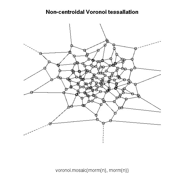
See also:
library(help=geometry) # qhull (convex hull, voronoi, etc.)
TODO
Bootstrap (Resampling)
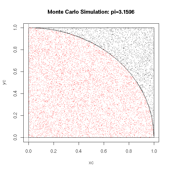
A "Monte Carlo Method" is any computation algorithm that relies on random numbers, whose result will change each time, whose result will be the more precise the more random numbers you use.
For instance, you can compute an approximate value of pi in the following way: take points at random (uniformly) in the [0,1]x[0,1] square and we count how many are in the dic of center 1 and center O. The ratio of that number over the total number of points is close to Pi/4.
pi.monte.carlo.plot <- function (n=10000, pch='.', ...) {
  x <- runif(n)
  y <- runif(n)
  interieur <- x^2 + y^2 <= 1
  p <- 4*sum(interieur)/n
  xc <- seq(0,1,length=200)
  yc <- sqrt(1-xc^2)
  plot( xc, yc, type='l' )
  lines( c(0,1,1,0,0), c(0,0,1,1,0) )
  abline(h=0, lty=3)
  abline(v=0, lty=3)
  points(x[interieur], y[interieur], col='red', pch=pch, ...)
  points(x[!interieur], y[!interieur], pch=pch, ...)
  title(main=paste("Monte Carlo Simulation: pi=",p,sep=''))
}
pi.monte.carlo.plot(100, pch='+', cex=3)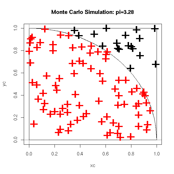
pi.monte.carlo.plot()
You can use it, as here, to compute multiple integrals. In small dimensions, it is not very useful (it is too slow), but in higher dimensions, it becomes more interesting. For instance, to compute an approximation of the integral of a function of 100 variables on the hypercube [0,1]^100, the rectangle method, i.e., computing the value of the function on each of the vertices of the hypercube, is not realistic, because there are 2^100 vertices; on the contrary, a Monte Carlo simulation vill give an acceptable value in a reasonable time.
Such simulations also enable you to compute the expectation of a given statistic (let us recall that a statistic is a function to be evaluated on a sample of a random variable, i.e., for a sample of dize n, a function R^m ---> R (to be absolutely rigorous, it is a family of such functions, one function for each sample size)). For instance, let us consider the following the following experiment: toss a die; if you get 1, draw a number at random from a gaussian distribution of mean -1 and standard deviation 1; otherwise, draw a number at random from a gaussian distribution of mean 1 and standard deviation 2; do this 10 times. What can you say of the mean, of the quartiles of those 10 numbers?
You could probably do the computation but, as we are lazy, let us ask the computer to perform a few simulations instead.
n <- 10
x <- ifelse( runif(n)>1/6, rnorm(n,1,2), rnorm(n,-1,1) )
mean(x)
quantile(x)
If you perform several such simulations, you get an estimation of the expectation of the mean of those numbers, and an estimation of the variance of the mean of those numbers.
n <- 10
N <- 1000
r <- matrix(NA, nr=N, nc=6)
for (i in 1:N) {
  x <- ifelse( runif(n)>1/6, rnorm(n,1,2), rnorm(n,-1,1) )
  r[i,] <- c( mean(x), quantile(x) )
}
colnames(r) <- c("mean", "0% (min)", "25%", "50% (median)", "75%", "100% (max)")
res <- rbind( apply(r,2,mean), apply(r,2,sd) )
rownames(res) <- c("mean", "sd")
It yields:
          mean  0% (min)        25% 50% (median)       75% 100% (max)
mean 0.6365460 -2.256153 -0.6387419    0.5499527 1.8228999   3.807241
sd   0.6446216  1.028375  0.7504127    0.7864454 0.8537194   1.236234
You can even ask some more and look at the distribution of the various statistics of interest.
n <- 10
N <- 1000
r <- matrix(NA, nr=N, nc=6)
for (i in 1:N) {
  x <- ifelse( runif(n)>1/6, rnorm(n,1,2), rnorm(n,-1,1) )
  r[i,] <- c( mean(x), quantile(x) )
}
colnames(r) <- c("mean", "0% (min)", "25%", "50% (median)", "75%", "100% (max)")
rr <- apply(r,2,density)
xlim <- range( sapply(rr,function(a){range(a$x)}) )
ylim <- range( sapply(rr,function(a){range(a$y)}) )
plot(NA, xlim=xlim, ylim=ylim, ylab='density')
for (i in 1:6) {
  lines(rr[[i]], col=i)
}
legend(par('usr')[2], par('usr')[4], xjust=1, yjust=1,
       c('mean', "min", "1st quartile", "median", "3rd quartile", "max"),
       lwd=1, lty=1,
       col=1:6 )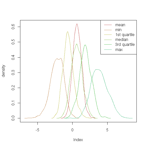
On this simulation, you see, in particular, that the mean and the median have more or less the same value, but the variance of the mean is lower, i.e., the mean is more precise. With such data, you would use the mean rather than the median.
To have an idea of the distribution of the statistic we are studying may help spot some pathologies. Thus, we ofthen assume that the statistics have an (almost) gaussian distribution. If you cannot (formally) prove this is the case, you can at least use simulations. In the following example, let us look at the quantile-quantile plots.
op <- par(mfrow=c(2,3))
for (i in 1:6) {
  qqnorm(r[,i], main=colnames(r)[i])
  qqline(r[,i], col='red')
  text( par("usr")[1], par("usr")[4], adj=c(-.2,2),
        round(shapiro.test(r[,i])$p.value, digits=4) )
}
par(op)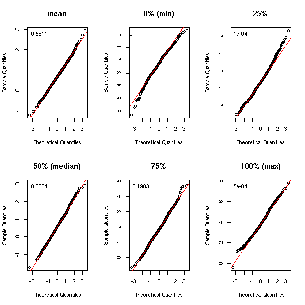
To avoid too much copy-pasting of the same code, let us use the following function for our simulations (in the following example, we look at the distribution of the coefficients of a regression).
my.simulation <- function (get.sample, statistic, R) {
  res <- statistic(get.sample())
  r <- matrix(NA, nr=R, nc=length(res))
  r[1,] <- res
  for (i in 2:R) {
    r[i,] <- statistic(get.sample())
  }
  list(t=r, t0=apply(r,2,mean))
}

r <- my.simulation(
  function () {
    n <- 200
    x1 <- rnorm(n)
    x2 <- rnorm(n)
    y <-  1 - x1 + 2 * x2 + rnorm(n)
   data.frame(y,x1,x2)
  },
  function (d) {
    lm(y~x1+x2, data=d)$coef
  },
  R=999
)

matdensityplot <- function (r, ylab='density', ...) {
  rr <- apply(r,2,density)
  n <- length(rr)
  xlim <- range( sapply(rr,function(a){range(a$x)}) )
  ylim <- range( sapply(rr,function(a){range(a$y)}) )
  plot(NA, xlim=xlim, ylim=ylim, ylab=ylab, ...)
  for (i in 1:n) {
    lines(rr[[i]], col=i)
  }
}

matdensityplot(r$t)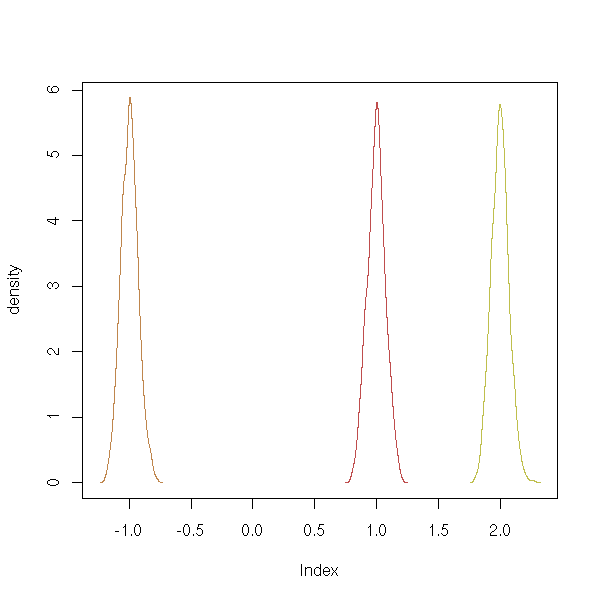
You can also use those simulations to study more complicated statistics, such as differences or quotients of means.
q <- runif(1,0,10)
m1 <- runif(1,0,10)
m2 <- q*m1
r <- my.simulation(
  function () {
    n1 <- 200
    n2 <- 100
    x1 <- m1*rlnorm(n1)
    x2 <- m2*rlnorm(n2)
    data.frame( x=c(x1,x2), c=factor(c(rep(1,n1),rep(2,n2))))
  },
  function (d) {
    a <- tapply(d[,1],d[,2],mean)
    a[2]/a[1]
  },
  R=999
)
hist(r$t, probability=T, col='light blue',
     main="Distribution of the ratio of two means")
lines(density(r$t), col='red', lwd=3)
abline(v=c(q,r$t0), lty=3, lwd=3, col=c('blue','red'))
legend( par("usr")[2], par("usr")[4], xjust=1, yjust=1,
        c("Theoretical mean", "Experimental mean"),
        lwd=1, lty=3, col=c('blue','red') )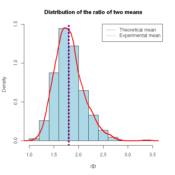
Instead of computing the mean and the standard deviation of our statistic, we can compute other quantities, such as confidence intervals or p-values.
# 5% confidence interval of the preceding example
hist(r$t, probability=T, col='light blue',
     main="Distribution of the ratio of two means")
qt <- quantile(r$t, c(.025,.975))
d <- density(r$t)
o <- d$x>qt[1] & d$x<qt[2]
lines(d$x[o], d$y[o], col='red', lwd=3)
lines(d, col='red')
abline(v=c(q,r$t0), lty=3, lwd=3, col=c('blue','red'))
legend( par("usr")[2], par("usr")[4], xjust=1, yjust=1,
        c("Theoretical mean", "Experimental mean",
          "5% confidence interval"),
        lwd=c(1,1,3), lty=c(3,3,1), col=c('blue','red', 'red') )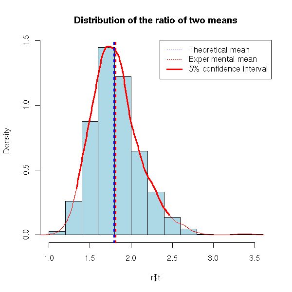
TODO: put the following code a bit later, in the section about
non-parametric bootstrap.
# We have two samples, of different sizes, and we study the
# quotient of their means
n1 <- 200
n2 <- 100
q <- runif(1,0,10)
m1 <- runif(1,0,10)
m2 <- q*m1
x1 <- m1*rlnorm(n1)
x2 <- m2*rlnorm(n2)
d <- data.frame( x=c(x1,x2), c=factor(c(rep(1,n1),rep(2,n2))))
R <- 999
library(boot)
r <- boot(d,
          function (d,i) {
            a <- tapply(d[,1][i],d[,2][i],mean)
            a[2]/a[1]
          },
          R=R)
hist(r$t, probability=T, col='light blue',
     main="Distribution of the ratio of two means")
qt <- quantile(r$t, c(.025,.975))
d <- density(r$t)
o <- d$x>qt[1] & d$x<qt[2]
lines(d$x[o], d$y[o], col='red', lwd=3)
lines(d, col='red')
abline(v=c(q,r$t0), lty=3, lwd=3, col=c('blue','red'))
legend( par("usr")[2], par("usr")[4], xjust=1, yjust=1,
        c("Theoretical mean", "Experimental mean",
          "5% confidence interval"),
        lwd=c(1,1,3), lty=c(3,3,1), col=c('blue','red', 'red') )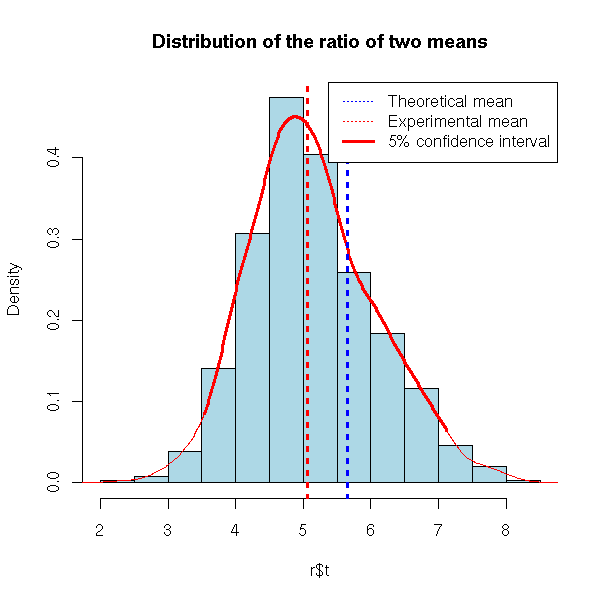
Simulations do not only study the distribution of the estimations of the model parameters, but also the distrinution of the predictions that use those estimated parameters.
TODO: an example
Compute the MDE for a classical regression

TODO: parametric bootstrap example, without "boot".

# The variables to predict are the first of the data.frame
my.simulation.predict <- function (
  get.training.sample,
  get.test.sample=get.training.sample,
  get.model,
  get.predictions=predict,
  R=999) {
  r <- matrix(NA, nr=R, nc=3)
  colnames(r) <- c("biais", "variance", "quadratic error")
  for (i in 1:R) {
    d.train <- get.training.sample()
    d.test <-  get.test.sample()
    m <- get.model(d.train)
    p <- get.predictions(m, d.test)
    if(is.vector(p)){ p <- data.frame(p) }
    d.test <- d.test[,1:(dim(p)[2])]
    b <- apply(d.test-p, 2, mean)
    v <- apply(d.test-p, 2, var)
    e <- apply((d.test-p)^2, 2, mean)
    r[i,] <- c(b,v,e)
  }
  list(t=r, t0=apply(r,2,mean))
}

get.sample <- function () {
  n <- 200
  x1 <- rnorm(n)
  x2 <- rnorm(n)
  y <- sin(x1) + cos(x2) - x1*x2 + rnorm(n)
  data.frame(y,x1,x2)
}
r <- my.simulation.predict(
  get.sample,
  get.model = function (d) {
    lm(y~x1+x2,data=d)
  }
)
hist(r$t[,1], probability=T, col='light blue',
     main="Bias of a linear regression")
lines(density(r$t), col='red', lwd=3)
abline(v=r$t0[1], lty=3)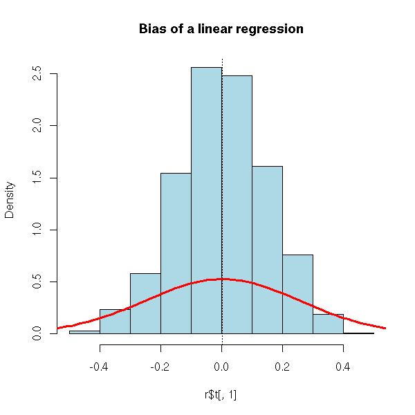
TODO: I am too allusive about the MSE. Recall what bias is, why
biased estimators are not necessarily bad.

TODO: another example for a biased method
(but we need something really biased)
Principal component regression? (or its continuous analogue, ridge regression)
You can use simulations to estimate the Mean Square Error (MSE) of several methods, in order to choose the best one.
get.sample <- function () {
  n <- 200
  x1 <- rnorm(n)
  x2 <- rnorm(n)
  y <- sin(x1) + cos(x2) - x1*x2 + rnorm(n)
  data.frame(y,x1,x2)
}
r1 <- my.simulation.predict(
  get.sample,
  get.model = function (d) {
    lm(y~x1+x2,data=d)
  }
)
r2 <- my.simulation.predict(
  get.sample,
  get.model = function (d) {
    lm(y~poly(x1,3)+poly(x2,3),data=d)
  }
)
library(splines)
r3 <- my.simulation.predict(
  get.sample,
  get.model = function (d) {
    lm(y~ns(x1)+ns(x2),data=d)
  }
)
matdensityplot(cbind(r1$t[,1], r2$t[,1], r3$t[,1]),
               main="Bias of three regression methods")
abline(v=c(r1$t0[1],r2$t0[1],r3$t0[1]), lty=3, col=1:3)
legend( par("usr")[2], par("usr")[4], xjust=1, yjust=1,
        c("Linear regression", "Polynomial regression", "Splines"),
        lty=1, lwd=1, col=1:3)
%--
This plot is not very helpful: let us look at the MSE.
> rbind( r1$t0, r2$t0, r3$t0 )
             bias  variance       MSE
[1,] -0.004572499  2.301057  2.311898
[2,] -0.001475014  2.186536  2.194847
[3,] -0.001067888  2.331862  2.342088
The second method seems preferable: the difference between the means is small but statistically significant.
> t.test( r2$t[,3], r1$t[,3] )
      Welch Two Sample t-test
data:  r2$t[, 3] and r1$t[, 3]
t = -7.1384, df = 1994.002, p-value = 1.317e-12
alternative hypothesis: true difference in means is not equal to 0
95 percent confidence interval:
 -0.14920930 -0.08489377
sample estimates:
mean of x mean of y
 2.194847  2.311898

> wilcox.test( r2$t[,3], r1$t[,3] )
      Wilcoxon rank sum test with continuity correction
data:  r2$t[, 3] and r1$t[, 3]
W = 397602, p-value = 3.718e-15
alternative hypothesis: true mu is not equal to 0
Here is another example, not to choose between different methods, but to estimate a parameter in a single method.
library(MASS)
get.sample <- function () {
  n <- 20
  x <- rnorm(n)
  x1 <- x + .2*rnorm(n)
  x2 <- x + .2*rnorm(n)
  x3 <- x + .2*rnorm(n)
  x4 <- x + .2*rnorm(n)
  y <- x + (x1+x2+x3+x4)/4 + rnorm(n)
  data.frame(y,x1,x2,x3,x4)
}
get.model <- function (d) {
  r <- lm.ridge(y~., data=d)
}
get.predictions <- function (r,d) {
  m <- t(as.matrix(r$coef/r$scales))
  inter <- r$ym - m %*% r$xm
  drop(inter) + as.matrix(d[,-1]) %*% drop(m)
}

lambda <- c(0,.001,.002,.005,.01,.02,.05,.1,.2,.5,1,2,5,10,20,50,100)
n <- length(lambda)
res <- rep(NA,n)
for (i in 1:n) {
  res[i] <- my.simulation.predict(
    get.sample,
    get.model = function (d) {
      lm.ridge(y~., data=d, lambda=lambda[i])
    },
    get.predictions = get.predictions,
    R=99
  )$t0[3]
}
plot(res~lambda, type='l', log='x')
abline(h=res[1], lty=3)
i <- (1:n)[ res == min(res) ]
x <- lambda[i]
y <- res[i]
points(x,y,col='red',pch=15)
title(main="Bootstrap simulations to choose the parameter in a ridge regression")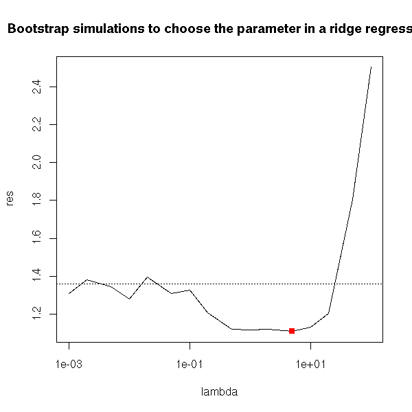
Maximum Likelihood Estimators are ofteh biased: the expectation of the estimator is not the right one. (However, the situation is not that bad: they are asymptotically unbiased, i.e., for large samples, the bias tends towards zero.)
TODO: give a biased MLE.
In other situations, the parameters might be unbiased, but the forecasts will be biased.
The estimators can even be intertionnaly biased: in ridge regression or in principal component regression, we accept a slight bias in exchange for a smaller variance, in the hope that it will decrease the MSE.
Simulations can help estimate the bias of an estimator of a forecast.
If we go back to the case of ridge regression, we realize that the forecasts are not really biased.
library(MASS)
get.sample <- function () {
  n <- 20
  x <- rnorm(n)
  x1 <- x + .2*rnorm(n)
  x2 <- x + .2*rnorm(n)
  x3 <- x + .2*rnorm(n)
  x4 <- x + .2*rnorm(n)
  y <- 1+x1+2*x2+x3+2*x4 + rnorm(n)
  data.frame(y,x1,x2,x3,x4)
}
get.model <- function (d) {
  r <- lm.ridge(y~., data=d)
}
get.predictions <- function (r,d) {
  m <- t(as.matrix(r$coef/r$scales))
  inter <- r$ym - m %*% r$xm
  drop(inter) + as.matrix(d[,-1]) %*% drop(m)
}

lambda <- c(0,.001,.002,.005,.01,.02,.05,.1,.2,.5,1,2,5,10,20,50,100)
lambda <- exp(seq(-7,7,length=100))
n <- length(lambda)
res <- rep(NA,n)
for (i in 1:n) {
  res[i] <- my.simulation.predict(
    get.sample,
    get.model = function (d) {
      lm.ridge(y~., data=d, lambda=lambda[i])
    },
    get.predictions = get.predictions,
    R=20
  )$t0[1]
}
plot(res~lambda, type='l', log='x')
abline(h=0,lty=3)
title("Bias in ridge regression forecasts")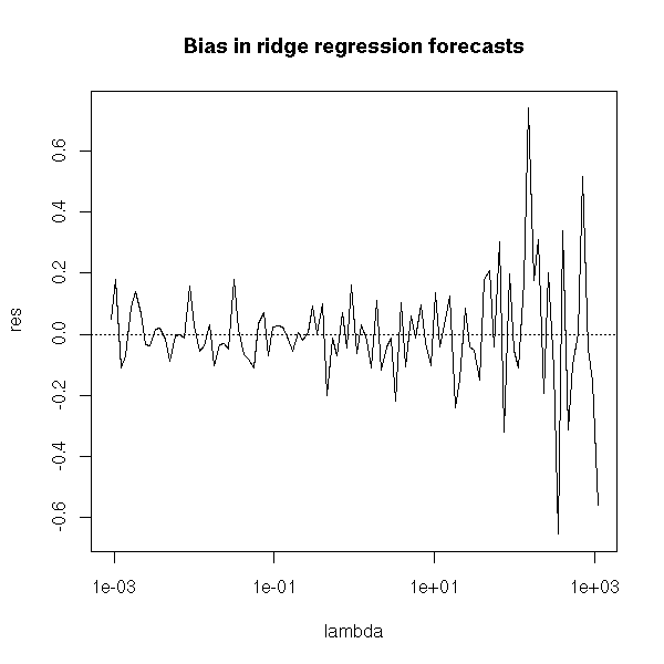
On the other hand, the estimation if the coefficients are biased.
get.sample <- function () {
  n <- 20
  x <- rnorm(n)
  x1 <- x + .2*rnorm(n)
  x2 <- x + .2*rnorm(n)
  x3 <- x + .2*rnorm(n)
  x4 <- x + .2*rnorm(n)
  y <- 1+2*x1+3*x2+4*x3+5*x4 + rnorm(n)
  data.frame(y,x1,x2,x3,x4)
}
s <- function(d,l) {
  r <- lm.ridge(y~., data=d, lambda=l)
  m <- t(as.matrix(r$coef/r$scales))
  inter <- r$ym - m %*% r$xm
  c(inter,m)
}
lambda <- exp(seq(-7,7,length=100))
n <- length(lambda)
res <- matrix(NA,nr=n,nc=5)
for (i in 1:n) {
  res[i,] <- my.simulation(
    get.sample,
    function (d) { s(d,lambda[i]) },
    R=20
  )$t0
}
matplot(lambda,res,type='l',lty=1,log='x')
abline(h=1:5,lty=3,col=1:5)
title("Bias in ridge regression coefficients")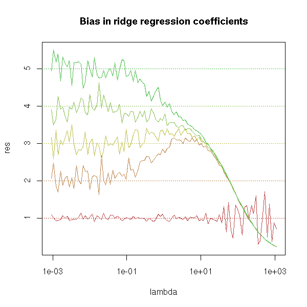
Let us take another example, Principal Component Regression (PCR) and let us plot the bias as a function of the parameter values.
get.sample <- function (a,b) {
  n <- 20
  x <- rnorm(n)
  x1 <- x + .2* rnorm(n)
  x2 <- x + .2* rnorm(n)
  y <- a*x1 + b*x2 + rnorm(n)
  data.frame(y,x1,x2)
}
get.parameters <- function (d) {
  y <- d[,1]
  x <- d[,-1]
  p <- princomp(x)
  r <- lm(y ~ p$scores[,1] -1)
  drop(p$loadings %*% c(r$coef,0))
}
N <- 5
a.min <- 0
a.max <- 10
res <- matrix(NA,nr=N,nc=N)
a <- seq(a.min,a.max,length=N)
b <- seq(a.min,a.max,length=N)
for (i in 1:N) {
  for(j in 1:N) {
    res[i,j] <- my.simulation(
      function () { get.sample(a[i],b[j]) },
      get.parameters,
      R=20
    )$t0[1] - a[i]
  }
}

persp(res)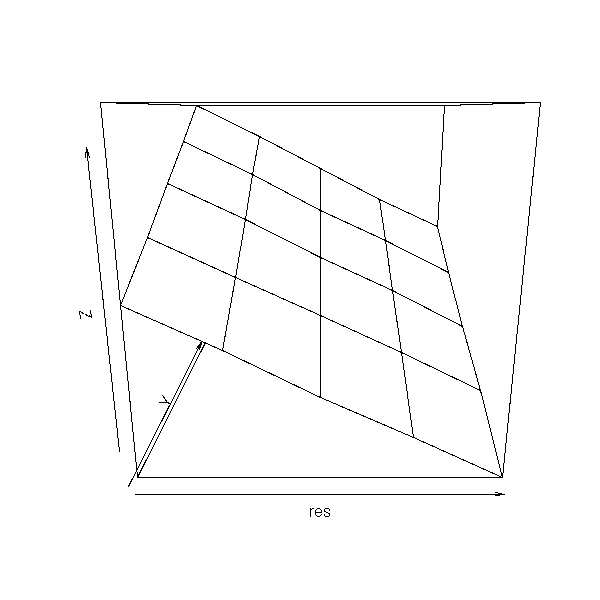
image(a,b,res,col=topo.colors(255))
text( matrix(a,nr=N,nc=N),
      matrix(b,nr=N,nc=N, byrow=T),
      round(res) )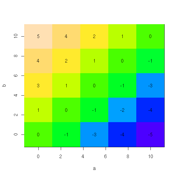
We can use this knowledge of the bias to help correct it. Thus, in the following example, the bias on a is approximately (b-a)/2.
get.parameters <- function (d) {
  y <- d[,1]
  x <- d[,-1]
  p <- princomp(x)
  r <- lm(y ~ p$scores[,1] -1)
  res <- drop(p$loadings %*% c(r$coef,0))
  a <- res[1]
  b <- res[2]
  c( a - (b-a)/2, b - (a-b)/2 )
}
N <- 5
a.min <- 0
a.max <- 10
res <- matrix(NA,nr=N,nc=N)
a <- seq(a.min,a.max,length=N)
b <- seq(a.min,a.max,length=N)
for (i in 1:N) {
  for(j in 1:N) {
    res[i,j] <- my.simulation(
      function () { get.sample(a[i],b[j]) },
      get.parameters,
      R=20
    )$t0[1] - a[i]
  }
}
persp(res)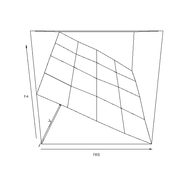
image(a,b,res,col=topo.colors(255))
text( matrix(a,nr=N,nc=N),
      matrix(b,nr=N,nc=N, byrow=T),
      round(res) )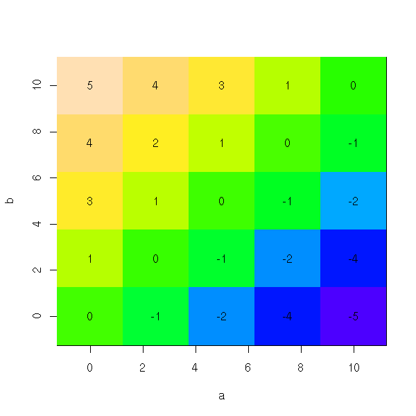
This is plain wrong: we get an estimation of the bias in function of the theoretical values of the parameters, while we would need an estimation of the bias as a function of their estimated values.
get.parameters <- function (d) {
  y <- d[,1]
  x <- d[,-1]
  p <- princomp(x)
  r <- lm(y ~ p$scores[,1] -1)
  drop(p$loadings %*% c(r$coef,0))
}
N <- 5
a.min <- 0
a.max <- 10
res <- matrix(NA,nr=N,nc=N)
res.a <- matrix(NA,nr=N,nc=N)
res.b <- matrix(NA,nr=N,nc=N)
a <- seq(a.min,a.max,length=N)
b <- seq(a.min,a.max,length=N)
for (i in 1:N) {
  for(j in 1:N) {
    r <- my.simulation(
      function () { get.sample(a[i],b[j]) },
      get.parameters,
      R=20
    )$t0
    res.a[i,j] <- r[1]
    res.b[i,j] <- r[2]
    res[i,j] <- r[1] - a[i]
  }
}
plot(res.a, res.b, type='n')
text(res.a, res.b, round(res))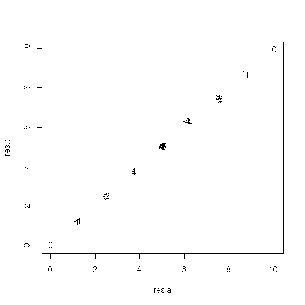
plot(as.vector(res) ~ as.vector(res.a-res.b))
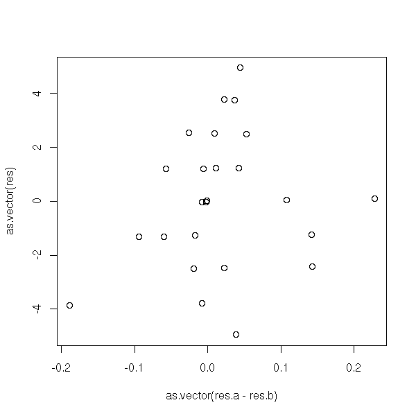
Well, that was not a very good example (but in some cases, such as ridge regression, above, estimating the bias and correcting it can improve the estimator).
In the preceding discussions, we assumed that we had a model that faithfully described the observations. In this case, we can usually compute exactly the expectation, the variance, the distribution of the estimators, their bias, their MSE.
However, those simulations, often called "parametric bootstrap" are still useful, in particular when the model is too complex for the exact computations to be carried out or when the model is given as a black box (say, you have a program to generate new observations, but you do not know how it works).
We shall now see that simulations can also be helpful even if we do not have a model: this is the "non-parametric bootstrap".
If we want to perform a simulation without any model (because we do not have any), with just the sample we have at hand, our only solution is to use this sample.
One of the first ideas to come to mind is to split the sample in two, using 75% of the data to find the estimator or the parameters needed for the forecasts, and using the 25 remaining percents to assess the quality of those forecasts. You can then repeat this process, with another splitting, in order to have a better idea of the distribution of the forecasting errors. Then, if the model or the algorithm seems acceptable, you run it on all the data (in order to have a more precise result that with the 75%). This is called cross-validation.
my.simulation.cross.validation <- function (
  s, # sample
  k, # number of observations to fit the the model
  get.model,
  get.predictions=predict,
  R = 999 )
{
  n <- dim(s)[1]
  r <- matrix(NA, nr=R, nc=3)
  colnames(r) <- c("bias", "variance", "MSE")
  for (i in 1:R) {
    j <- sample(1:n, k)
    d.train <- s[j,]
    d.test <-  s[-j,]
    m <- get.model(d.train)
    p <- get.predictions(m, d.test)
    if(is.vector(p)){ p <- data.frame(p) }
    d.test <- d.test[,1:(dim(p)[2])]
    b <- apply(d.test-p, 2, mean)
    v <- apply(d.test-p, 2, var)
    e <- apply((d.test-p)^2, 2, mean)
    r[i,] <- c(b,v,e)
  }
  list(t=r, t0=apply(r,2,mean))
}

n <- 200
x1 <- rnorm(n)
x2 <- rnorm(n)
x3 <- rnorm(n)
y <- 2 - x1 - x2 - x3 + rnorm(n)
s <- data.frame(y,x1,x2,x3)
r <- my.simulation.cross.validation(s, 150, function(s){lm(y~.,data=s)}, R=99)
hist( r$t[,3], probability=T, col='light blue',
      main="MSE estimation by cross-validation" )
lines(density(r$t[,3]),col='red',lwd=3)
abline(v=mean(r$t[,3]),lty=2,lwd=3,col='red')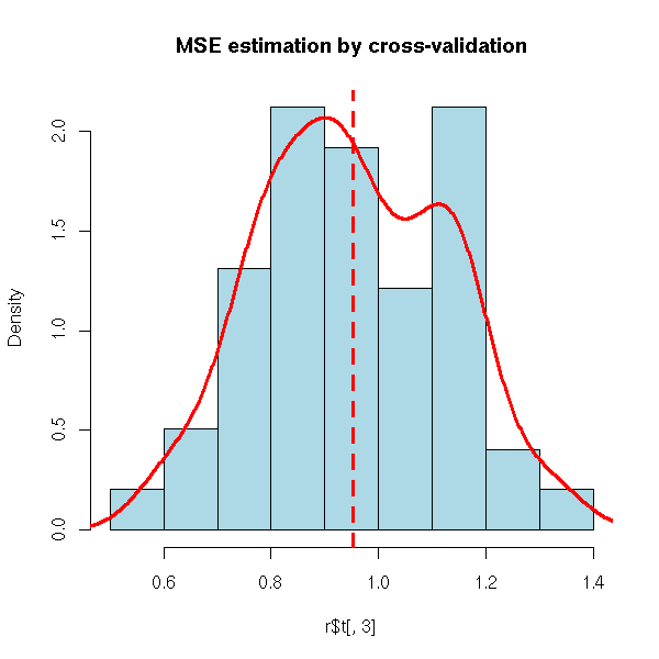
The splitting need not be 75%/25%, you can take 90%/10% or even remove a single observation: this is the Kack-knife.
my.simulation.jackknife <- function (
  s,
  get.model,
  get.predictions=predict,
  R=999)
{
  n <- dim(s)[1]
  if(R<n) {
    j <- sample(1:n, R)
  } else {
    R <- n
    j <- 1:n
  }
  p <- get.predictions(get.model(s), s)
  if( is.vector(p) ) {
    p <- as.data.frame(p)
  }
  r <- matrix(NA, nr=R, nc=dim(s)[2]+dim(p)[2])
  colnames(r) <- c(colnames(s), colnames(p))
  for (i in j) {
    d.train <- s[-i,]
    d.test <-  s[i,]
    m <- get.model(d.train)
    p <- get.predictions(m, d.test)
    r[i,] <- as.matrix(cbind(s[i,], p))
  }
  r
}

n <- 200
x1 <- rnorm(n)
x2 <- rnorm(n)
x3 <- rnorm(n)
y <- 2 - x1 - x2 - x3 + rnorm(n)
s <- data.frame(y,x1,x2,x3)
r <- my.simulation.jackknife(s, function(s){lm(y~.,data=s)})
hist( r[,5]-r[,1], col='light blue' )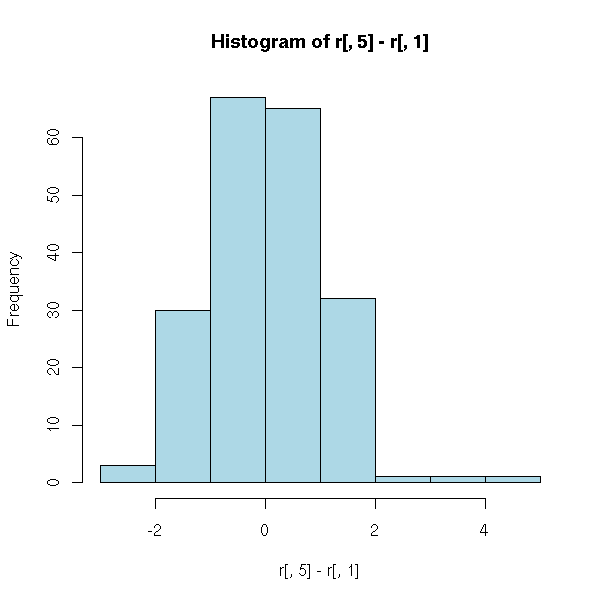
TODO: explain how to lower the bias of an estimator with the Jackknife.

TODO
Explain the idea, give the resulting formula, and finally the
formula actually used.

TODO
Give an example (probably the population variance, which is a biased
estimator: the jack-knife will give the sample variance).
In crossed validation (or in the jack-knife), each observation was used exactly once: you build the sample on which you will perform the computations by sampling WITHOUT replacement. Instead, you can sample WITH replacement: this os the idea behind the bootstrap. In other words, the sample is used as an infinite population.
We choose to sample WITH replacement so that the random variables be independant -- when you sample without replacement, they are not.
To implement this, we could reuse the function we had used for cross-validation.
my.simulation.bootstrap <- function (
  s,
  get.model,
  get.predictions=predict,
  R = 999 )
{
  n <- dim(s)[1]
  r <- matrix(NA, nr=R, nc=3)
  colnames(r) <- c("bias", "variance", "MSE")
  for (i in 1:R) {
    j <- sample(1:n, n, replace=T)
    d.train <- s[j,]
    d.test <-  s
    m <- get.model(d.train)
    p <- get.predictions(m, d.test)
    if(is.vector(p)){ p <- data.frame(p) }
    d.test <- d.test[,1:(dim(p)[2])]
    b <- apply(d.test-p, 2, mean)
    v <- apply(d.test-p, 2, var)
    e <- apply((d.test-p)^2, 2, mean)
    r[i,] <- c(b,v,e)
  }
  list(t=r, t0=apply(r,2,mean))
}

n <- 200
x1 <- rnorm(n)
x2 <- rnorm(n)
x3 <- rnorm(n)
y <- 2 - x1 - x2 - x3 + rnorm(n)
s <- data.frame(y,x1,x2,x3)
r <- my.simulation.bootstrap(s, function(s){lm(y~.,data=s)}, R=99)
hist( r$t[,3], col='light blue',
      main="Using the bootstrap to estimate the MSE" )
lines(density(r$t[,3]),col='red',lwd=3)
abline(v=mean(r$t[,3]),lty=2,lwd=3,col='red')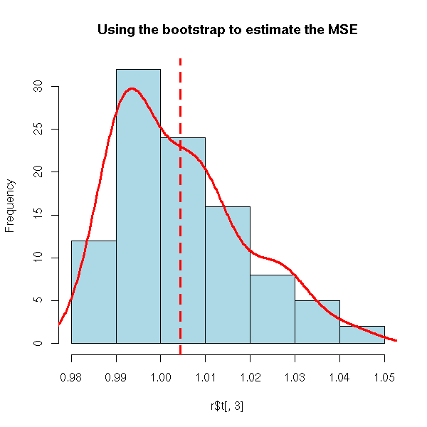
But actually, there is already a function to do this.
Here is, for instance, our first application of the bootstrap: investigate the distribution of a statistic (here, the mean of a sample).
library(boot)
n <- 200
x <- rlnorm(n)
r <- boot(x, function(s,i){mean(s[i])}, R=99)
hist(r$t, probability=T, col='light blue')
lines(density(r$t),col='red',lwd=3)
abline(v=mean(r$t),lty=2,lwd=3,col='red')
title("Bootstrap to estimate the distribution of the mean of a sample")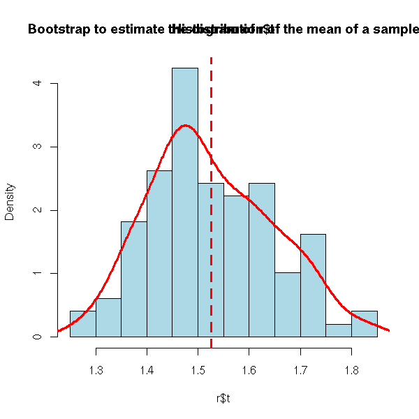
The first argument contains the observations, as a vector (if there is only one variable), an array or a data.frame. The second argument is the statistic, as a function whose arguments are the data and the vector of indices and that returns a vector. The last argument is the number of bootstrap samples to consider (at least 1,000).
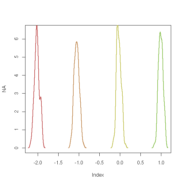
n <- 200
x1 <- rnorm(n)
x2 <- rnorm(n)
x3 <- rnorm(n)
y <- -2 - x1 +0* x2 + x3 + rnorm(n)
s <- data.frame(y,x1,x2,x3)
r <- boot(s, function(s,i){lm(y~.,data=s[i,])$coef}, R=99)
plot(NA,xlim=range(r$t), ylim=c(0,6.5))
for (i in 1:4) {
  lines(density(r$t[,i]), lwd=2, col=i)
}
The result is a list. We shall mainly be interested in two of ots components: t, that contains all the estimations of the statistic and t0, that contains the same estimation for the whole sample. The "print.boot" function also gives the estimated bias.
> r
ORDINARY NONPARAMETRIC BOOTSTRAP
Call:
boot(data = s, statistic = function(s, i) {
    lm(y ~ ., data = s[i, ])$coef
}, R = 99)
Bootstrap Statistics:
      original        bias    std. error
t1* -2.0565761 -0.0001888077  0.06901359
t2* -1.0524309 -0.0060001140  0.06248444
t3* -0.1340356 -0.0082527142  0.06299820
t4*  1.0176907  0.0013180553  0.06206947
Let us now consider the other application of the bootstrap: assessing the quality of forecasts. Here, we merely study the statistic "MSE of the forecasts".
n <- 200
x1 <- rnorm(n)
x2 <- rnorm(n)
x3 <- rnorm(n)
y <- 1+x1+x2+x3+rnorm(n)
d <- data.frame(y,x1,x2,x3)
r <- boot(d,
          function (d,i) {
            r <- lm(y~.,data=d[i,])
            p <- predict(r, d[-i,])
            mean((p-d[,1][-i])^2)
          },
          R=99)
hist(r$t,probability=T,col='light blue',
     main="Mean Square Error (MSE)")
lines(density(r$t),lwd=3,col='red')
abline(v=mean(r$t),lty=3)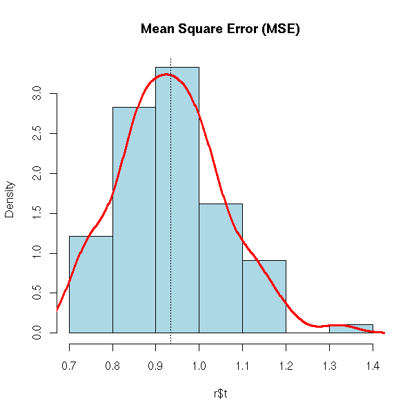
The belief underlying the bootstrap is the following: the relation between the sample at hand and the population it comes from is very similar to those between the sample at hand and the bootstrap samples we draw from it (i.e., the samples sampled with replacement from the sample at hand).
Let us check on an example that this assumption is not too unrealistic.
get.sample <- function (n=50) { rnorm(n) }
get.statistic <- function (x) { mean(x) }
# Plot the density of the estimator
R <- 200
x <- rep(NA,R)
for (i in 1:R) {
  x[i] <- get.statistic(get.sample())
}
plot(density(x), ylim=c(0,4), lty=1,lwd=3,col='red',
     main="Relevance of the bootstrap")
# Let us plot a few estimations of this density,
# obtained from the bootstrap
for (i in 1:5) {
  x <- get.sample()
  r <- boot(x, function(s,i){mean(s[i])}, R=R)
  lines(density(r$t))
}
curve(dnorm(x,sd=1/sqrt(50)),add=T, lty=2,lwd=3,col='blue')
legend(par('usr')[2], par('usr')[4], xjust=1, yjust=1,
       c('parametric bootstrap', 'non-parametric bootstrap',
         "theoretical curve"),
       lwd=c(3,1,2),
       lty=c(1,1,2),
       col=c("red", par("fg"), "blue"))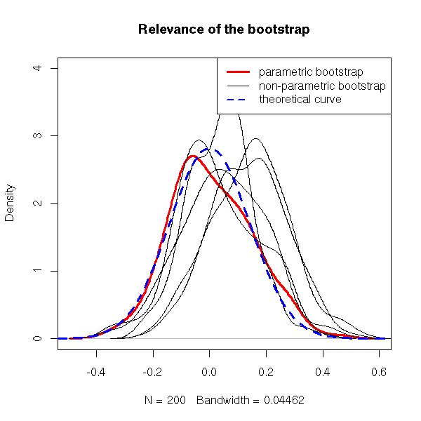
Conclusion: do not expect any miracle from the bootstrap.
The bootstrap is only relevant for some, "well-behaved", estimators: in particular, avoid it to study pathological estimators such as the maximum.
n <- 50
x <- rnorm(n)
r <- boot(x, function(s,i){max(s[i])}, R=999)
hist(r$t, probability=T, col='light blue',
     main="A statistic for which the bootstrap is not very relevant...")
lines(density(r$t,bw=.05), col='red', lwd=3)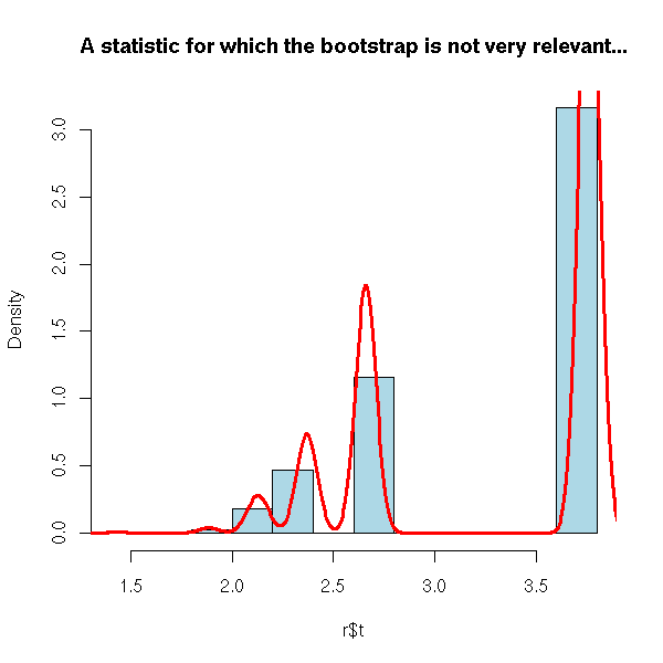
The "boot.ci" function derives confidence intervals from bootstrap results.
n <- 20
x <- rnorm(n)
r <- boot(x, function(x,i){mean(x[i])}, R=99)

> boot.ci(r)
BOOTSTRAP CONFIDENCE INTERVAL CALCULATIONS
Based on 99 bootstrap replicates

CALL:
boot.ci(boot.out = r)

Intervals:
Level      Normal              Basic
95%   (-0.1457,  0.6750 )   (-0.2429,  0.5969 )

Level     Percentile            BCa
95%   (-0.1050,  0.7348 )   (-0.0559,  0.7891 )
Calculations and Intervals on Original Scale
Some basic intervals may be unstable
Some percentile intervals may be unstable
Warning: BCa Intervals used Extreme Quantiles
Some BCa intervals may be unstable
Warning messages:
1: Bootstrap variances needed for studentized intervals in: boot.ci(r)
2: Extreme Order Statistics used as Endpoints in: norm.inter(t, adj.alpha)

n <- 20
N <- 100
r <- matrix(NA,nr=N,nc=2)
for (i in 1:N) {
  x <- rnorm(n)
  r[i,] <- boot.ci(boot(x,function(x,i){mean(x[i])},R=99))$basic[c(4,5)]
}
plot(NA,xlim=c(-1.5,1.5), ylim=c(0,2),
     main="Confidence interval boundaries (bootstrap)")
lines(density(r[,1]), lwd=3, col='red')
lines(density(r[,2]), lwd=3, col='blue')
abline(v=0,lty=3)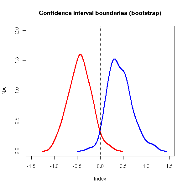
The bootstrap is biased towards zero, because some observations are used both on the sample used to build the model (i.e., the bootstrap sample) and in the sample used to validate it (i.e., the whole initial sample, used as the population).
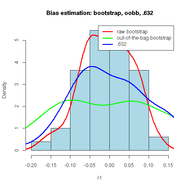
The "out-of-the-bag bootstrap" and the ".632 bootstrap" try to correct this bias.
The out-of-the-bag bootstrap does not use all the observations to validate the model, but only those that were not in the bootstrap sample -- this is already what we were doing with cross-validation.
Actually, the out-of-the-bag bootstrap is still biased, but in the other directions. To correct this bias, one can consider a weighted mean of the raw bootstrap and the oob bootstrap.
.368 * (bias estimated from the raw bootstrap) +
  .632 * (bias estimated from the oob bootstrap)
This strange ".632" coefficient comes from the following remark: when the sample size is large, the bootstrap samples contain on average 63.2% of the initial observations.
TODO: example?
The following example is not very good: the estimator is not
biased...

n <- 200
x1 <- rnorm(n)
x2 <- rnorm(n)
x3 <- rnorm(n)
y <- 1+x1+x2+x3+rnorm(n)
d <- data.frame(y,x1,x2,x3)
r1 <- boot(d, function (d,i) {
             r <- lm(y~.,data=d[i,])
             p <- predict(r, d)
             mean(p-d[,1])
           },
           R=99)$t
r2 <- boot(d, function (d,i) {
             r <- lm(y~.,data=d[i,])
             p <- predict(r, d[-i,])
             mean(p-d[,1][-i])
           },
           R=99)$t
r3 <- .368*r1 + .632*r2
hist(r1,probability=T,col='light blue',
     main="Bias estimation: bootstrap, oobb, .632")
lines(density(r1),lwd=3,col='red')
lines(density(r2),lwd=3,col='green')
lines(density(r3),lwd=3,col='blue')
legend(par('usr')[2], par('usr')[4], xjust=1, yjust=1,
       c("raw bootstrap", "out-of-the-bag bootstrap", ".632"),
       lwd=3,
       col=c("red", "green", "blue")
      )
In the context of a linear regression, one tends to bootstrap the residuals rather than the observations.
You can see this as a semi-parametric bootstrap.
In a parametric bootstrap, you would choose a model (here, a linear model with gaussian noise), estimate the parameters of this model (the linear relation and the noise variance) and sample from that model.
Here, you only choose half a model: a linear model with unspecified noise. You estimate the model (the linear relation) and sample from the estimated noise (the residuals).
TODO
plot( res ~ leverage )

library(boot)
fit <- lm(calls ~ year, data=phones)
ph <- data.frame(phones, res=resid(fit), fitted=fitted(fit))
ph.fun <- function(data, i) {
  d <- data
  d$calls <- d$fitted + d$res[i]
  coef(update(fit, data=d))
}
ph.lm.boot <- boot(ph, ph.fun, R=499)
ph.lm.boot
The bootstrap cannot be directly applied to time series because the observations are not independant. Usually, one samples (with replacement) chunks of time series and joins them together.
If the time series looks like an AR(1) process, one would rather do that the first difference of the time series.
TODO: in the above examples, use the "boot" function, even for the parametric bootstrap.
get.sample.ridge <- function (n=100) {
  x1 <- rnorm(n)
  x2 <- rnorm(n)
  y <- 1 - x1 - x2 + rnorm(n)
  data.frame(y,x1,x2)
}
statistic.ridge <- function (x, lambda=0) {
  r <- lm.ridge(y~x1+x2, data=x, lambda=lambda)
}
statistic.ridge.for.boot <- function (x,i, lambda=0) {
  statistic.ridge(x[i,], lambda=10)
}

# Non-parametric bootstrap
n <- 20
N <- 100
x <- get.sample.ridge()
r <- boot(x, statistic.ridge.for.boot, R=999)
It yields:
> r
ORDINARY NONPARAMETRIC BOOTSTRAP
Call:
boot(data = x, statistic = statistic.ridge.for.boot, R = 999)
Bootstrap Statistics:
      original       bias    std. error
t1*  1.1380068 0.0007701467  0.10555253
t2* -1.0200495 0.0037754155  0.09702321
t3* -0.9293355 0.0017206597  0.08876848
And for the parametric bootstrap:
# Parametric bootstrap
ran.ridge <- function (d, p=c(1,-1,-1)) {
  n <- 100
  x1 <- rnorm(n)
  x2 <- rnorm(n)
  y <- p[0] + p[1]*x1 - p[2]*x2 + rnorm(n)
  data.frame(y,x1,x2)
}
r <- boot(x, statistic.ridge.for.boot, R=999, sim='parametric',
          ran.gen=ran.ridge, mle=c(1,-1,-1))
TODO: There is an error...
TODO: estimating the bias for biased forecasts (take a classical regression, do the forecasts and add 1 -- so as to be sure the forecasts are biased). Use the "boot" function for those forecasts.
Plot the forecast error density for the chosen method before and after correction of the bias.
TODO: compare several regressions.
y <- sin(2*pi*x)+.3*rnorm(n)
y~x
y~ns(x)
y~poly(x,20)
Compare: MSE (bootstrap), AIC, BIC
- Split the observations into 10 groups: 1, 2, ..., 10.
- Use groups 2,3,...,10 to compute the estimator, compare with group 1,
  estimate the bias.
- Repeat with groups 1,3,4...,10 (i.e., put aside group 2),
  etc.
  The mean of those 10 biases is an estimation of the bias.
- Compute the estimator with thw whole sample, correct it with the
  estimated bias.
TODO: reuse the following paragraph.
Consider the following situation. We have a sample, from a non-gaussian population, and we are trying to estimate a statistic (mean, median, maximum, the coefficients of a regression, etc.). Which estimator should we choose? Is it biased? Can we have an estimation of thi bias? What is its variance? Has it a gaussian distribution? Can we have confidence intervals? If we do not know anything of the whole population, we cannot say much. But we do know something: we have a sample. The idea is to use this sample to manufacture more samples (we simply sample, with replacement, from this sample -- this differs from cross-validation where we sample without replacement). As we now have several samples, we can study the behaviour and the relevance of the various candidate estimators
TODO: recall that one cannot study ANY statistic that way. For the results to be correct/meaningful/relevant, it has to have some theoretical properties. The typical pathological example is the "maximum".
TODO: completely rewrite what follows. With another example -- the maximum is the worst you could think of...
TODO: Bias and optimism.
Let us explain the difference between bias and optimism. We have a population (which we do not know), a sample, and several bootstrap samples. We also have an estimator, supposed to measure some parameter of the population. The bias of this estimator is the expectation of the difference between this parameter and its estimation from the sample; the optimism is the difference between the estimator evaluated on the sample and the average of its evaluations on the bootstrap samples.
The bias is a comparison between the parameter and the estimator, the optimism is a comparison of the estimator between the sample and the bootstrap samples (the optimism completely forgets about the parameter to be estimated).
TODO: write a funtion to perform bootstrap computations.

my.bootstrap <- function (data, estimator, size, ...) {
  values <- NULL
  n <- dim(data)[1]
  for (i in 1:size) {
    bootstrap.sample <- data[ sample(1:n, n, replace=T), ]
    values <- rbind(values, t(estimator(bootstrap.sample, ...)))
  }
  values
}
TODO: present the "boot" function. Already done above (The "bootstrap" package is older.)
library(boot)
my.max <- function (x, i) { max(x[i]) }
r <- boot(faithful$eruptions, my.max, R=100)
plot(r)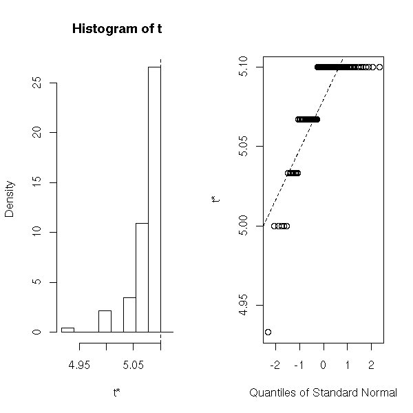
> r

ORDINARY NONPARAMETRIC BOOTSTRAP

Call:
boot(data = faithful$eruptions, statistic = my.max, R = 100)

Bootstrap Statistics:
    original   bias    std. error
t1*      5.1 -0.02265   0.0367342
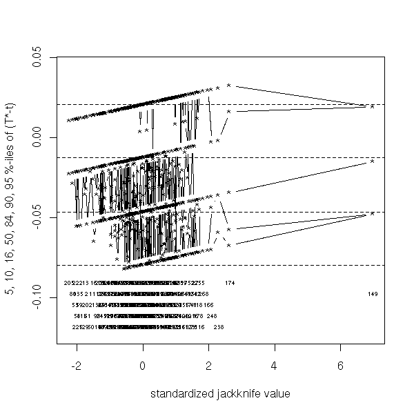
I do not know what it is. (to investigate the influence of each observation on the result).
TODO
jack.after.boot(r)
The efficiency of the bootstrap relies on the belief that the relation between the population (that we do not know) and the sample (we have one) is the same as the relation between the sample and the bootstrap samples. There is no reason for those relations to be exactly the same.
To try to justify the bootstrap, we can perform the following experiment.
1. Choose a distribution
2. Take a sample
3. Apply the bootstrap to estimate a parameter of confidence
   intervals.
4. Go back to point 2.
Here is what it could yield:
TODO...
TODO: compare parametric and non-parametric bootstrap (in particular, look how many samples you must have to get reliable estimators).
TODO: already done above...
TODO: delete/proofread this example
get.sample <- function (n=50) {
  x <- rnorm(n)
  y <- 1-x+rnorm(n)
  data.frame(x,y)
}
s <- get.sample()

R <- 100
n <- dim(s)[1]
x <- s$x
y <- s$y
res <- rep(NA,R)
res.oob <- rep(NA,R)
for (k in 1:R) {
  i <- sample(n,n,replace=T)
  xx <- x[i]
  yy <- y[i]
  r <- lm(yy~xx)
  ip <- rep(T,n)
  ip[i] <- F
  xp <- x[ip]
  yp <- predict(r,data.frame(xx=xp))
  try( res.oob[k] <- sd(yp - s$y[ip]) )
  res[k] <- sd( yy - predict(r) )
}
plot(density(res), main="Basic and out-of-the-box bootstrap")
lines(density(res.oob),lty=2)
abline(v=1,lty=3)
legend( par("usr")[2], par("usr")[4], xjust=1, yjust=1,
        c("Basic bootstrap", "Out-of-the-box bootstrap"),
        lwd=1, lty=c(1,2) )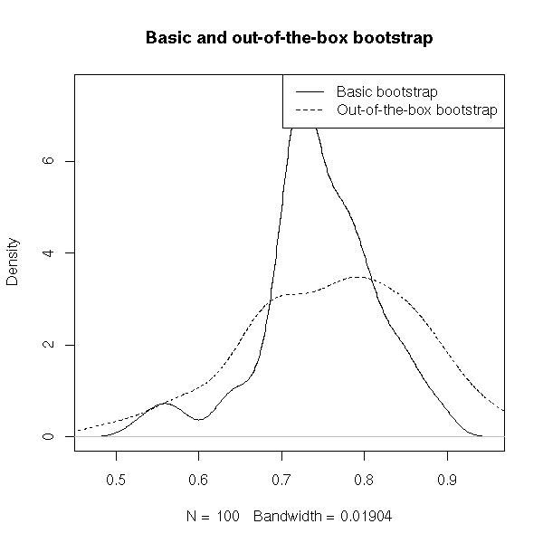
It yields
> mean(res)
[1] 0.9221029

> mean(res.oob)
[1] 0.9617512
instead of 1. In most cases, however, classical bootstrap gives overoptimistic estimations while the oob bootstrap is too pessimistic: quite often, we take a (weighted) mean of both.
> .368*mean(res) + .632*mean(res.oob)
[1] 0.9471606
TODO: proofread this
TODO: change the title of this section?
We have seen how the bootstrap could help us estimate the bias, variance and MSE of an estimator. It allows us to compare several estimators and choose the "best" (say, the one with the lowest MSE).
We have already tackled the same problem with ridge regression: if the variables are multicolinear, a regression using
b = (X'X)^-1 X' y
would not work well (because the X'X matrix is almost singular: the estimator would have a higes variance); instead we use
b = (X'X + kI)^-1 X' y.
Let us try to find the value of k that minimizes the estimator variance. (In this situation, as there is nothing but linear algebra and gaussian distributions, you probably can do the exact computations.)
echantillon.multicolineaire <- function (n=100) {
  x0 <- rep(1,n)
  x1 <- x0 + .1*rnorm(n)
  x2 <- x0 + .1*rnorm(n)
  x3 <- x0 + .1*rnorm(n)
  y <- x0 + x1 + x2 + x3 + rnorm(n)
  x <- cbind(x0,x1,x2,x3)
  m <- cbind(y,x)
  m
}
m <- echantillon.multicolineaire()
f <- function (m, k) {
  x <- m[,-1]
  y <- m[,1]
  n <- dim(x)[2]
  solve( t(x) %*% x + k*diag(rep(1,n)), t(x) %*% y )
}
N <- 200
variance <- rep(NA, N)
biais <- rep(NA, N)
exact <- f(m,0)
k <- exp(seq(.01,4, length=N))-1
for (j in 1:N) {
  g <- function (m, i) { f(m[i,], k[j]) }
  s <- boot(m, g, R=1000)
  variance[j] <- max(var(s$t))
  biais[j] <- max(exact - apply(s$t,2,mean))
}
plot(variance ~ k, log='x', type='l')
par(new=T)
plot(biais ~ k, type='l', log='x', col='red', xlab='', ylab='', axes=F)
axis(4, col="red")
legend( par("usr")[2], par("usr")[4], yjust=1, xjust=0,
        c("variance", "optimism"),
        lwd=1, lty=1,
        col=c(par('fg'), 'red') )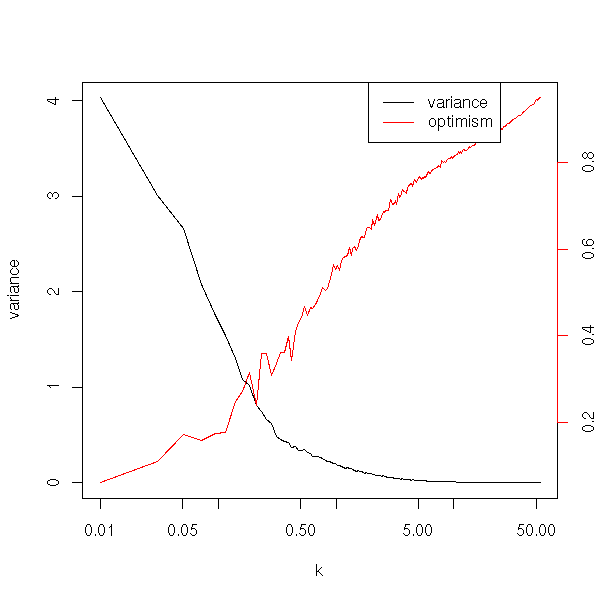
TODO: This plot does not suggest k=10... Before using the "boot" function, I got:
my.bootstrap <- function (data, estimator, size, ...) {
  values <- NULL
  n <- dim(data)[1]
  for (i in 1:size) {
    bootstrap.sample <- data[ sample(1:n, n, replace=T), ]
    values <- rbind(values, t(estimator(bootstrap.sample, ...)))
  }
  values
}

n <- 100
x0 <- rep(1,n)
x1 <- x0 + .1*rnorm(n)
x2 <- x0 + .1*rnorm(n)
x3 <- x0 + .1*rnorm(n)
y <- x0 + x1 + x2 + x3 + rnorm(n)
x <- cbind(x0,x1,x2,x3)
f <- function (m, k) {
  x <- m[,-1]
  y <- m[,1]
  n <- dim(x)[2]
  solve( t(x) %*% x + k*diag(rep(1,n)), t(x) %*% y )
}
N <- 200
variance <- rep(NA, N)
biais <- rep(NA, N)
k <- exp(seq(0,6, length=N))-1
for (i in 1:N) {
  s <- my.bootstrap(cbind(y,x), f, 100, k[i])
  variance[i] <- max(apply(s, 2, var))
  biais[i] <- max(abs( s -
    matrix( as.vector(f(cbind(y,x),0)), nr=dim(s)[1], nc=dim(s)[2], byrow=T )
  ))
}
plot(variance ~ k, log='x', type='l')
par(new=T)
plot(biais ~ k, type='l', log='x', col='red', xlab='', ylab='', axes=F)
axis(4)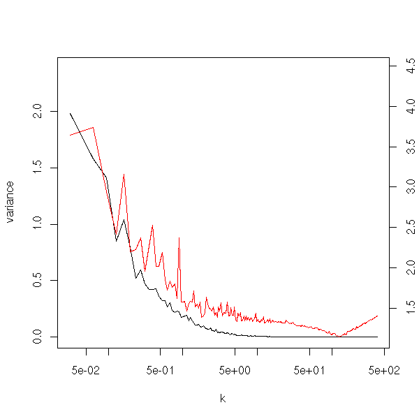
We choose k=0.2
> g <- function (m, i) { f(m[i,], .2) }
> s <- boot(m, g, R=100)
> apply(s$t,2,mean)
[1] 1.1294813 1.0082432 0.3821003 1.2957629

> g <- function (m, i) { f(m[i,], 10) }
> s <- boot(m, g, R=100)
> apply(s$t,2,mean)
[1] 0.9402689 0.9762665 0.8696934 0.9346982
These values are much better that those obtained with k=0 (i.e., with classical regression): the coefficients of x1, x2, x3 are supposed to be equal.
> as.vector(exact)
[1] 1.3112394 1.0350861 0.2463275 1.2259999
We can check the forecasts accuracy.
s <- my.bootstrap(cbind(y,x), f, 100, 10)
b <- apply(s, 2, mean)
b0 <- as.vector(f(cbind(y,x),0))

# Another sample from the same population
# TODO: put this in a function
n <- 100
x0 <- rep(1,n)
x1 <- x0 + .1*rnorm(n)
x2 <- x0 + .1*rnorm(n)
x3 <- x0 + .1*rnorm(n)
y <- x0 + x1 + x2 + x3 + rnorm(n)
x <- cbind(x0,x1,x2,x3)

a1 <- x %*% b
a2 <- x %*% b0
boxplot( c(as.vector(a1), as.vector(a2)) ~
         gl(2,n,2*n, c("ridge", "classic")),
         horizontal=T )
title(main="Residues of a ridge regression")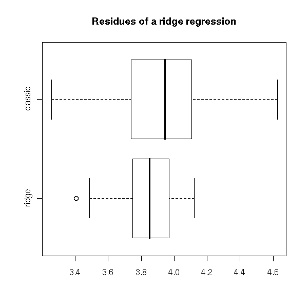
library(ipred)
Sample use of the bootstrap
95% confidence band for spline regression
Compare with the confidence intervals provided by classical
regression.
We have just used regression to compare estimators, we can also use
it to compare models.
TODO: For each bootstrap example, add a few plots:
boxplot, hist, qqnorm, jack.after.boot
boot.ci to compute confidence intervals (several methods, some
require very long computations).
TODO: To sort
An article about the bootstrap and its implementation in R in
http://cran.r-project.org/doc/Rnews/Rnews_2002-3.pdf

library(help=bootstrap)
Old

library(help=boot)
More recent
Also works with right-censored data and time series.
?censboot
?tsboot
Also: multi-sample problems

TODO: influence function estimation from the bootstrap.
?empinf
The estimators obtained from the Maximum Likelihood method are often biased (they are asymptotically unbiased, though). The Jack-Knife algorithm can transform a biased estimator U into a less-biased one.
Split the sample into N samples of the same size (for instance, of size 1) and compute the estimatior Ui on each of those samples. Then, set
J = N U - (N-1)/N * (U1 + U2 + ... + Un)
For instance, if we start with the population variance formula (the one with "n" in the denominator, which is a biased estimator), we get the sample variance formula (with "n-1" in the denominator: it is unbiased).
TODO: check this.
TODO
library(boot)
?jack.after.boot
Use the bootstrap to:
estimate the variance of an estimator
compute a confidence interval
perform tests, compute p-values
Example: take a sample, bootstrap to get a 95% confidence interval. Plot, as a function of the bootstrap sample, the median median and the 0.025 and 0.975 quantiles of the median.
TODO
TODO
# Use bootstrap (normal or .632) or cross-validation
# to estimate classification error
library(ipred)
?errortest
xpdf ipred-examples.pdf
TODO: Should this really be here???
TODO: plot 1:

The forecast error (on the taring sample and the test
sample) as a function of the model complexity. When a
model is too complex, the forecasts are bad: this is
called overfit.)

n <- 50
k <- 10
N <- 50
get.sample <- function (n) {
  x <- runif(n)
  y <- sin(2*pi*x)+.3*rnorm(n)
  m <- data.frame(x=x, y=y)
  m
}
error <- rep(NA,k)
for (i in 1:k) {
  e <- rep(NA,N)
  for (j in 1:N) {
    training.sample <- get.sample(n)
    x <- training.sample$x
    y <- training.sample$y
    r <- lm(y~poly(x,i))
    test.sample <- get.sample(1000)
    e[j] <- mean( (predict(r, data.frame(x=test.sample$x)) - test.sample$y)^2 )
  }
  error[i] <- mean(e)
}
plot(error, type='l', log='y',
     xlab="Model complexity",
     ylab="Errorr")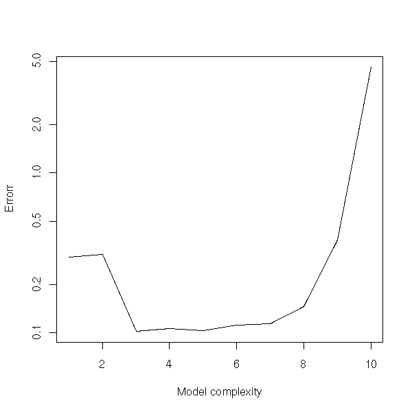
We can plot bias, variance, Mean Squared Error (MSE) as a function of the model complexity, the parameter in ridge regression, the number of neighbours in the "k nearest nearest neighbours" method, the speed at which the temperature decreases in simulated annealing, the number of parameters in principal component regression, the degree in polynomial regression, the number of nodes in restricted cubic splines, etc.
TODO: detail
a <- 2
curve(dnorm(x-a), xlim=c(-3,5), ylim=c(0,.5))
abline(v=0, lty=3, col='red')
abline(v=a, lty=3, col='blue')
arrows(0,.45,a,.45, code=3, col='green')
arrows(a-pnorm(1), dnorm(pnorm(1)), a+pnorm(1), dnorm(pnorm(1)), code=3, col='red')
legend(par('usr')[2], par('usr')[4], xjust=1,
       c("true value", "estimator expectation", "bias", "variance"),
       lwd=1, lty=c(3,3,1,1),
       col=c('red', 'blue', 'green', 'red') )
title(main="Bias and variance of a biased estimator")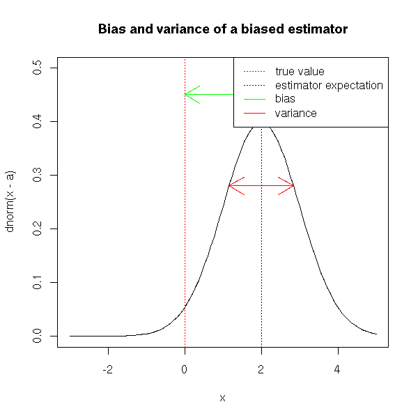
The algorithm is clearly described here:
http://students.washington.edu/~fkrogsta/bayes/stat538.pdf
For more details, Google for "MCMC metropolis hastings".
Motivations
  Random sampling
  Integral computations (expectation: mean, varaince, etc.)
  Bayesian Methods
  Examples of spaces
Metropolis Algorithms, Implementation
Generalizations and variants
  Hastings corrections
  Gibbs sampling
  Metropolis-Hastings-Green
Applications
  Phylogeny
  Multiple Alignment
We want to sample at random an element among the population (x1,x2,...,xn) according to the distribution (p1,p2,...,pn). A very complicated way of doing so consists in designing a Markov chain whole limit distribution is (p1,...,pn).
For simple examples, it is really weird, but you sometimes face finite but huge spaces (or "universes"): for instance, in a phylogenetic study, you might want to sample from the set of 1000-leaf trees.
If we wanted an equi-probable distribution, we could find a simpler way out: but, in order to perform simulations, we would like the trees to describe the evolution of the species we are studying, we would like the more probable trees to appear more often and the more unlikely ones to appear more rarely.
But the situation is even worse that that! Usuallky, we cannot compute the probability of each element. For each tree a, we can compute a score S(a) and the probability of a tree a0 is
           score(a0)
P(a0) = ----------------
          Sum score(a)
           a
The problem is that the sum at the denominator has too many terms to be computed.
Markov chains will allow us to wander in the space of all trees, going from a tree to a "neighbouring" tree (for a notion of "neighbourhood" still to be defined). The samples wil will get on that way will not be independant, but they will be sufficient to computes quantities of interest associated to the probability distribution on our space of trees.
One meets those non-equiprobable probability measures when one applies bayesian methods: when we want to compute the value of a parameter in a model, the values that best fits the observed data data, we often ask for a single result. But this is not natural, because the result will be imprecise: often, we complete this result with a "variance". This variance is meaningful if the distribution of the estimated parameter is gaussian, which is rarely the case (it can be skewed, it can be bimodal -- or even worse, the parameter need not be a number, it could be a tree in a huge set of trees). An idea, to get around this problem, is to give, not a single value of the parameter but all its distribution: if we really want a single value, if we think (after having a look at the distribution, to check if it is a good idea), we can take the mode (this will be a Maximum Likelohood (ML) estimator) or the mean of this distribution; if we want confidence intervals, having the distribution will yield more accurate results. This distribution is known as the "a posteriori" (or "posterior" distribution).
If the universe is intricate (e.g., if it is a set of trees or graphs), it might be hard to describe this probability distribution. But that is not a problem, because we do not need to describe it: if we can randomly sample from it, we can easily get the answer to our questions (mode, median, confidence intervals, etc.). The methods we are about to present are actually (Monte Carlo simulations with Markov Chains, MCMC) will allow us to perform suc a sampling.
The Monte Carlo method allows you to compute an integral
Integral( f(x), x \in I )
in the following way: take x1, x2,..., xn at random in I and compute
 1
---   Sum    f(X_k)
 N   k=1..N
If the set I over which we integrate is a close interval of the real line, we shall draw x1 at random from a uniform distribution. On the contrary, if it is the whole real line, it will not work (there is no uniform probability distribution on the whole real line). Instead, we shall try to write the function to integrate under the form f(x) = g(x) p(x) where p is the density of a probability distribution on the real line. Then, we just have to sample the xi from that distribution and compute
 1
---    Sum   g(X_k)
 N   k=1..N
If you compare this with the classical numerical integration algorithmas you are used to (rectangles, etc.), it does not seem very efficient -- especially in dimension 1, i.e., if you integrate a function of a single variable. Monte Carlo integration becomes more interesting in higher dimensions. Imagine you want to compute the integral of a function f of 1000 variables in the hypercube [0,1]^1000. The generalization of the rectangles method suggests to evaluate the function at each vertex of this hypercube and average those values. The problem is that this hypercube has 2^1000 vertices. This is too much. Instead, the Monte Carlo method will just evaluate f at a few hundred points in the hypercube and average them: it is not as precise, but we do not have to wait until the Sun becomes a super nova.
This example might sound extreme: do we really see functions of a thoud variables in our day to day life? Do we really have to compute integral on such spaces in concrete problems?
Well, yes, we do. With a phylogenetic tree describing the evolution of a thousand species, you might want to know the number of mutations on each of the branches, i.e., the length of those branches. The set of those lengths (a thousand) is a point in a high-dimension space. Actually, the situation is even worse, because you will want to consider all the possible trees...
But do we really want to compute integrals on such spaces? Well, yes, we do: mean (expectation), variance, probabilities can be expressed as integrals. For instance, the probability that the situation we are studying is in a set H0 of hypotheses, given that we we observed O is:
P(H \in H0) = integral( P(H|O), H \in H0 )

                         P(O|H) P(H)
            = integral( ------------- , H \in H0 )
                            P(O)
Other example: the probability of observing O given that we have already observed O is
P(O'|O) = Integral( P(O'|H) * P(H|O), H )
Here is a simplistic algorithm:
For i = 1 to N:
  Choose Xi at random following the distribution p
The problem is that p can be arbitrary and, in particular, diffucult to compute. In the situations we shall be interested in, the universe will be finite but very large and the probabilities will be of the form
               w(a)
P(X=a) = ------------------
           Sum( w(b), b )
We can compute the numerator, but the denominator, a sum onver all the elements of the universe, cannot be computed.
Instead, we can try:
Choose X0 at random
For i = 1 to N:
  Choose Xi among the neighbours of X(i-1)
In other words, we put a Markov chain on our space, that allows us to jump from an element x(i) to another nearby x(i+1). The way we define that notion of "neighbouring element" is called a "transition kernel".
There is a slight problem, however: we no longer use p. Let us put it back in.
Choose X0 at random
For i = 1 to N:
  Choose X' among the neighbours of X(i-1)
  Set X(i) = X(i-1) or X(i) = X' (choose according to p)
But how do we "choose according to p"? As p has the form mentionned above, we cannot compute the probability of a given element, but we can compute the quotent of two such probabilities. We can proceed as follows.
# Metropolis Algorithm
Choose X0 at random
For i = 1 to N:
  Choose X' among X(i-1)'s neighbours
  Choose a number u at random in [0,1]
            P(X')
  If u < -----------
          P(X(i-1))
  Then
    X(i) = X'
  Else
    X(i) = X(i-1)
This algorithm works (i.e., the Markov chain has the desired limit distribution) if (the transition network satisfies a few properties and) the Markov chain is symetric, i.e., if the probability of going from X to Y is the same as that of going from Y to X. If not, the algorithm has to be amended, as follows.
# Metropolis-Hastings Algorithm
Choose X0 at random
For i = 1 to N:
  Choose X' among X(i-1)'s neighbours
  Choose a number u, uniformly at random in [0,1]
          P( X(i-1) | X' )     P(X')
  If u < ------------------ -----------
          P( X' | X(i-1) )   P(X(i-1))
  Then
    X(i) = X'
  Else
    X(i) = X(i-1)
You might have a few qualms about the Xi's not being independant -- but actually, it is not that serious.
P(X | X') only depends on the distance between X and X'.
In the algorithm, we can change
Choose X' among X(i-1)'s neighbours
into
Choose X' at random.
If the distribution used to choose X' has fatter tails than the target distribution, it will work fine -- but otherwise, it will not.
In an n-dimensional space, we can change the coordinates one at a time.
According to the literature, it is simpler, more rudimentary than the Metropolis-Hastings: but to me, it seems more complex and besides, it assumes you know much more about the distribution.
The Gibbs sampler is a particular case of the preceding method, that tackled one coordinate at a time: but here, we ash that the transition kernel be the conditionnal probability
P(xi | xj, j!=i)
It means that we have to know those conditionnal probabilities...
Let us consider, for instance, two random variables X1, X2, gaussian, with zero mean, variance 1, covariance r. Then, we have
X1|X2 ~ N(r*X2, 1-r^2)
and similarly for X2. At each step of the algorith, we either modify X1 or X2. The path is thus "manhattanian".
my.gibbs <- function (x0=c(0,0), N=20, r=.5, plot.it=T) {
  res <- matrix(NA, nr=N, nc=2)
  res[1,] <- c(0,0)
  for (i in seq(2,N-1,by=2)) {
    x1 <- res[i-1,1]
    x2 <- res[i-1,2]
    res[i,2] <- x2
    # WE are supposed to take the new point at random
    # and accept or reject it depending of the conditionnal
    # probability.
    # Here, I directly sample from the conditionnal probability.
    x1 <- rnorm(1, r*x2, sd=sqrt(1-r^2))
    res[i,1] <- x1
    res[i+1,1] <- x1
    x2 <- rnorm(1, r*x1, sd=sqrt(1-r^2))
    res[i+1,2] <- x2
  }
  if (plot.it) {
    plot(res, type='l', xlab="x1", ylab="x2", main="Gibbs sampler")
    points(res, pch=16)
    invisible(res)
  } else {
    res
  }
}
my.gibbs()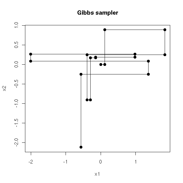
my.gibbs(N=1000)
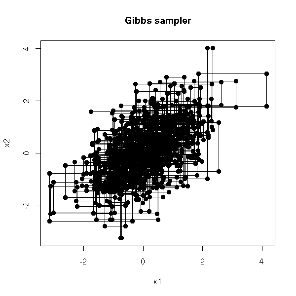
With the Metropolis-Hastings, a path would rather look like
r <- my.gibbs(N=40,plot.it=F)[2*(1:20),]
plot(r, type='l', xlab="x1", ylab="x2",
     main="Path of a Metropolis simulation (almost)")
points(r, pch=16)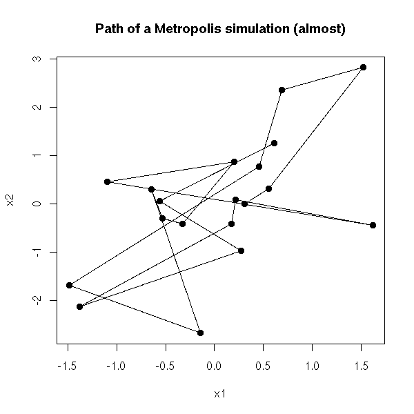
r <- my.gibbs(N=2000,plot.it=F)[2*(1:1000),]
plot(r, type='l', xlab="x1", ylab="x2",
     main="Path of a Metropolis simulation (almost)")
points(r, pch=16)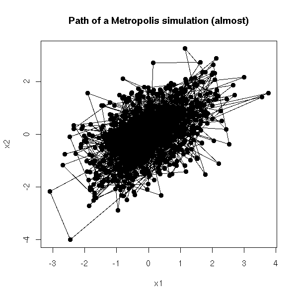
TODO: An example that shows that the general appearance of the paths do not depend on the starting point (plot two paths, with completely different starting points, in two different colors).
We are studying a family of proteins (a protein is a sequence of amino acids, i.e., a string of characters written with a 20-letter alphabet) and we are looking for a pattern common to this family.
To simplify, let us assume that we are looking for a pattern of length L (the length is known in advance). We start by taking a segment of length L on each of the sequences: the set of those segments is a (very bad) first approximation of our pattern.
Then, at each step of the algorithm, we choose one of the sequences and we check all the possible positions of the window of length L: we choose the best (variant: we choose one at random, with a probability proportionnal to its score; variant: simulated annealing).
A few problems can occur: you have to choose the width of the window; if you run the algorithm several times, you will not get the same result (are they variants of the same pattern? overlapping patterns? completely different patterns?)
See:
http://www.msci.memphis.edu/%7Egiri/compbio/papers/gibbs2.pdf
Consider a model of the form
X = f(Y1,Y2)
where Y1 and Y2 are independant. We have observed X and we are trying to predict Y1 from X. For instance:
Y1 = The stalion has a certain gene
Y2 = The mare has this gene
X  = The offspring has the gene
We shall use the Gibbs sampler to predict both Y1 and Y2.
Here Y1 and Y2 are the model parameters: in those methods, parameters and random variables play the same role.
We first choose initial (random) values for Y1 and Y2. Then, we compute
                P(X | Y1,Y2) * P(Y1 | Y2)
P(Y1 | X,Y2) = ---------------------------
                      P(X | Y2)

                P(X | Y1,Y2) * P(Y1)
             = ----------------------     (because Y1 and Y2 are independant)
                    P(X | Y2)
This is possible, because we know the model, this allows us to sample at random a new value for Y1.
We start again with Y2.
We iterate, many times: after a while, the algorithm has reache its stationnary regime and the values of Y1 and Y2 we get follow the posterior distribution of those parameters: we can use them to compute the mode (the mean, the median or any other relevant information) of Y1.
TODO: give an example, with computations in R.
Exercise: implement a Gibbs sample to find the mean and the variance of a sample supposed to follow a gaussian distribution.
TODO

P(mean | X, variance) = ...
P(variance | X, mean) = ...
This is a generalization of the Metrolopis--hastings in which we replace the probability densities by (non-necessarily continuous) probability distributions: this generalizes all the variants above, including the Gibbs sampler.
The choice of the transition kernel (i.e., the notion of neighbourhood) is delicate.
First, we must accept new values quite often, otherwise, we could get stuck in a point. For this, the "neighbours" have to be rather "near".
On the other hand, in order to reach quite quickly states rather far away, we would need "neighbours" that are not too near...
In order to see wether those problems occur, in order to choose (or parametrize) the transition kernel, we can make a few plots. In dimension one, these plots are simply the time series plot, the AutoCorrelation Function (ACF) and the Partial AutoCorrelation Function (PACF). The ACF will also help us build independant variables, by taking X(n), X(n+k), X(n+2k), X(n+3k), etc., with k sufficient large so that the autocorrelation cor(X(n),X(n+k)) be sufficiently small.
One should also perform several simulations, with different starting points, in order to see if the algorithm converges or not and, more importantly, how long it takes to converge. A single longer simulation might also be useful to check the convergence.
N <- 200
K <- 5
res <- matrix(NA, nr=N, nc=K)
for (i in 1:K) {
  r <- my.gibbs(x0=runif(2,-1,1), N=N, plot.it=F)
  res[,i] <- apply(r,1,cumsum)[1,] / 1:N
}
matplot(res, type='l', lty=1,
        ylab="Estimator", xlab="Simulation length",
        main="Gibbs sampler")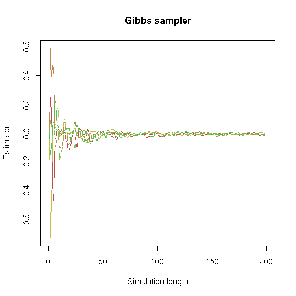
Usually, we discard the start of the time series, the "burn-in" phase, so that the Markov chain reaches its stationnary distribution.
In R:
library(ts)
MH <- function (N = 1000,
                voisin = function (x) { rnorm(1,x,1) },
                p = dnorm,                 # Probability distribution to simulate
                q = function (x,y) { 1 }   # Hastings Correction
               ) {
  res <- rep(NA,N)
  x <- 0
  for (i in 1:N) {
    y <- voisin(x)
    u <- runif(1)
    if ( u < q(x,y)/q(y,x) * p(y)/p(x) ) {
      x <- y
    }
    res[i] <- x
  }
  ts(res)
}

x1 <- ts(rnorm(1000))
x2 <- MH()
x3 <- MH(voisin = function (x) { rnorm(1,x,.01) })
x4 <- MH(voisin = function (x) { rnorm(1,x,50) })

op <- par(mfrow=c(4,1))
plot(x1, main="Random")
plot(x2, main="MCMC")
plot(x3, main="MCMC, neighbours too near")
plot(x4, main="MCMC, neighbours too far")
par(op)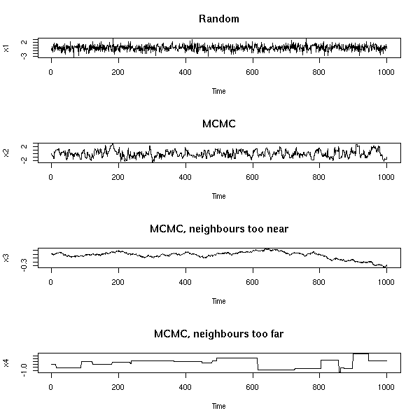
op <- par(mfrow=c(2,2))
qqnorm(x1, main="Random"); qqline(x1);
qqnorm(x2, main="MCMC"); qqline(x2);
qqnorm(x3, main="MCMC, neighbours too near"); qqline(x3);
qqnorm(x4, main="MCMC, neighbours too far away"); qqline(x4)
par(op)
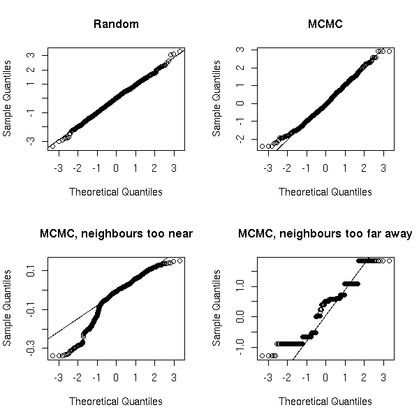
op <- par(mfrow=c(2,2))
hist(x1, col='light blue', probability=T, main="Random")
curve(dnorm(x),col='red',lwd=3, add=T)
hist(x2, col='light blue', probability=T, main="MCMC")
curve(dnorm(x),col='red',lwd=3, add=T)
hist(x3, col='light blue', probability=T, main="MCMC, neighbours too near")
curve(dnorm(x),col='red',lwd=3, add=T)
hist(x4, col='light blue', probability=T, main="MCMC, neighnours too far away")
curve(dnorm(x),col='red',lwd=3, add=T)
par(op)
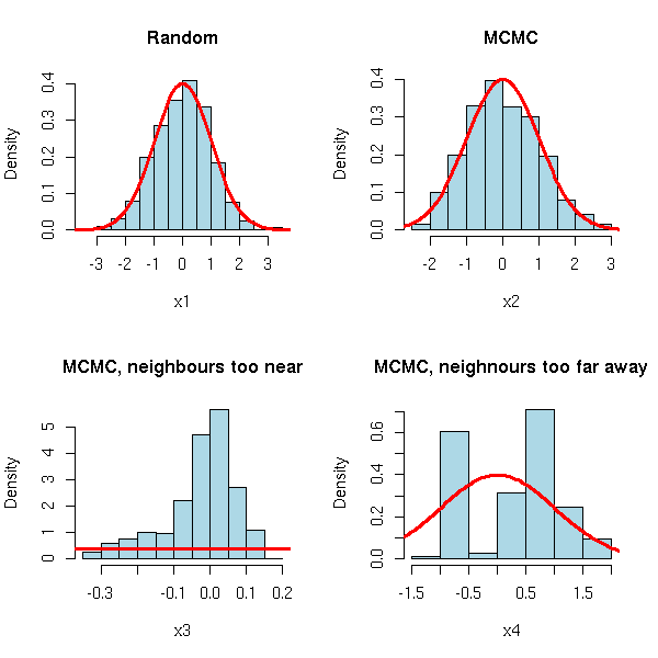
op <- par(mfrow=c(4,1))
acf(x1, main="Random")
acf(x2, main="MCMC")
acf(x3, main="MCMC, neighbours too near")
acf(x4, main="MCMC, neighnours too far away")
par(op)
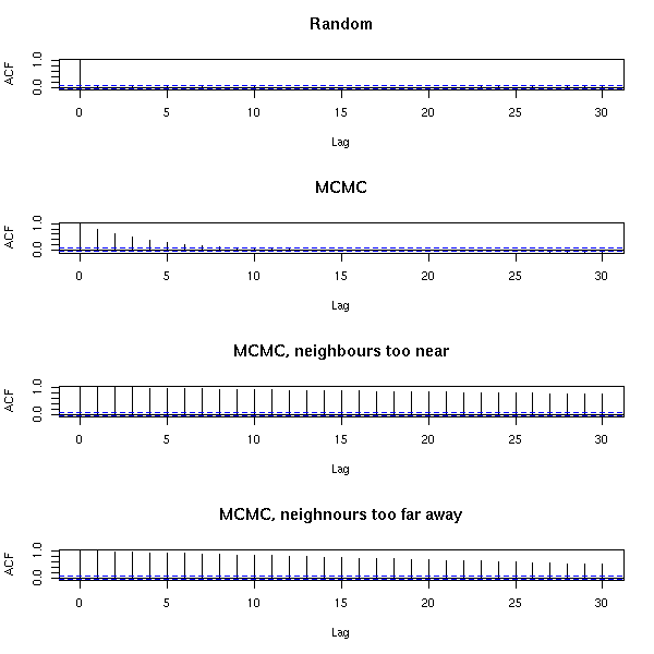
op <- par(mfrow=c(4,1))
pacf(x1, main="Random")
pacf(x2, main="MCMC")
pacf(x3, main="MCMC, neighbours too near")
pacf(x4, main="MCMC, neighnours too far away")
par(op)
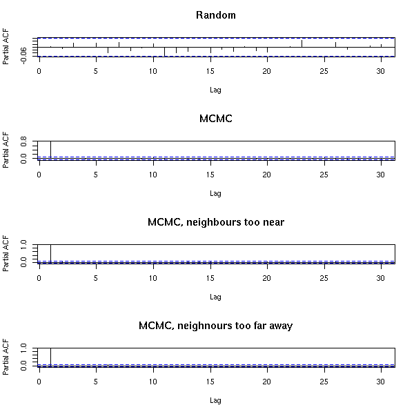
For an order-1 Markov chain, it is normal: all the information we want is in the first autocorrelation.
Application to an integral computation (this is the variance of a standard gaussian distribution: it should be 1):
> mean(x1^2)
[1] 0.960904
> mean(x2^2)
[1] 1.004407
> mean(x3^2)
[1] 0.01575253
> mean(x4^2)
[1] 0.9143307
Other example: we can use this Markov chain to have iid random variables following the distribution in question. We cannot directly take the values we get because they are not independant -- the is the gist of Markov chains: we can jump from one value to the next -- it is all but independant.
N <- 3000
x <- MH(N=N)
plot(x[2:N]~x[2:N-1],xlab='x(i)',ylab='x(i+1)')
abline(0,1,col='red')
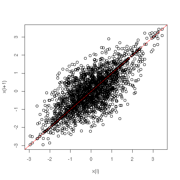
The horizontal line comes from the rejection of some values: in this case, we have two successive identical values.
On the contrary, if we take one value out of 10 or 100, it looks random.
N <- 100000
x <- MH(N=N)
x <- x[100:length(x)]  # burn-in
x <- x[seq(1,length(x),by=50)]
N <- length(x)
plot(x[2:N]~x[2:N-1],xlab='x(i)',ylab='x(i+1)')
abline(0,1,col='red')
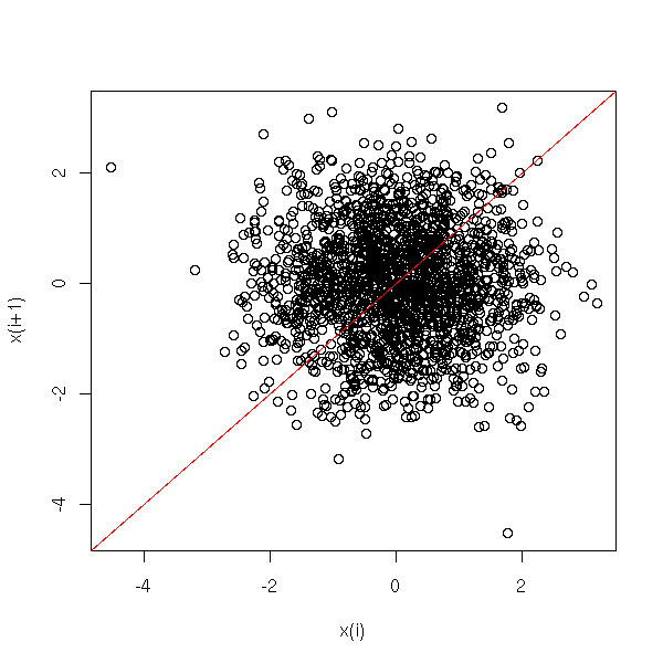
op <- par(mfrow=c(4,1))
plot(ts(x))
acf(x)
pacf(x)
spectrum(x)
par(op)
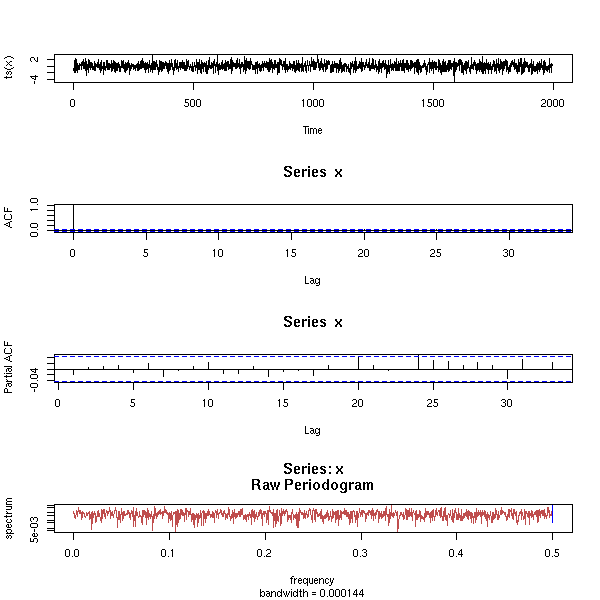
On the MCMC algorithms, we can change the probability of accepting a new state as the algorithm proceeds: at first, we are very lenient, we accpet states we should not really accept and progressively, we get closer to the Metrolopis-Hastings probability.
This may help circumvent some pathologies of the Markov chain (irreducibility, etc.).
We can modify this idea to fit a completely different goal: maximizong (or minimizing) some function, for instance, a log-likelihood. The algorithm (called "simulated annealing") is the following:
1. Take a value at random
2. Take a new value "near" the old one.
3. If it is better,
   Then
     Keep the value
   Else
     Keep the old value, with a certain probability
4. Go to 2.
A very, very long time a go, I wrote about optimization algorithms, including simulated annealing:
http://zoonek.free.fr/Ecrits/1994_recuit_simule.ps.gz
To estimate a paramter of a statistical model with the Maximum Likelohood Method, we have to compute a "log-likelihood", that will be a sum (or an integral, it is the same thing). If this sum is too large, we can use Monte Carlo methods to estimate it.
TODO
In order to compute
I = Integral( f(x) p(x), x \in I )
when we do not know how to sample elements from the distribtion defined by p, we can try to write
                       p(x)
I = Integral( f(x) * ------ * q(x), x \in I )
                       q(x)
where q defines a distribution for which we can easily sample.
One can use this method even if we know p, because if we carefully choose q (namely, if q is larger at the places where f changes (i.e., where we need more precision) and smaller where f does not change much (i.e., when we can afford less precision)), we can lower the variance of I.
http://galton.uchicago.edu/%7Eeichler/stat24600/Handouts/l9.pdf
TODO: explain what it is (Gibbs sampling)
TODO: list of available software
  OpenBUGS (new version of WinBUGS, that was only available under Windows)
  JAGS
  Hydra
From a user's point of view, the idea is the following: we have an intuition of how the data was generated or, more reasonably, of how we could generate similar data. This intuition is a general process, that depends on parameters we do not know: we want to estimate those parameters. You can see those parameters as hidden variables.
This sounds very much like maximum likehood estimation (or any other way of building estimators), but there is a difference: we also have some vague information about those parameters. More precisely, we consider them as random variables, with a known distribution (for instance, if we know that a parameter is always in the interval [0,1], this distribution could be the uniform distribution on this interval; if we know that the parameter is "around zero and not too large", we this distribution could be a gaussian distribution with mean 0 and variance 1; if we know that the parameter is "around zero, often with large values", this distribution could be a Cauchy distribution).
Here is an example:
Parameters:
  a is taken from a gaussian distribution N(0,1)
  b is taken from a gaussian distribution N(0,1)
  v is taken from a lognormal distribution LN(0,1)
Observations:
  x[1],...,x[n] are taken from iid random variables N(0,1)
  e[1],...,e[n] are taken from iid random variables N(0,v)
  for (i in 1:n) {
    y[n] <- a + b * x[n] + e[n]
  }
konqueror http://mathstat.helsinki.fi/openbugs/Software.html
wget http://mathstat.helsinki.fi/openbugs/OpenBUGSRTApril5.zip
unzip *zip
cd OpenBUGS/
chmod +x cbugs
Ahhhhh....
It is not written in C or C++ but in Oberon (well, a successor of Oberon). There is no makefile. They provide "Linux executable" -- as if they were processor-independant. Well, the executable is not executable (this may be due to their choice of the ZIP format for the archive).
There are also redistribution restrictions (it is built on non-free libraries):
Some of the subdirectories in the OpenBUGS distribution
only contain /Code and /Rsrc subdirectories. These are the
libraries provided by Oberonmicrosystem. The symbol files
and documentation for these libraries are included with
the BlackBox tools. Oberonmicrosystems only allows the
/Code and /Rsrc subdirectories of these libraries to
be distributed!
The instructions to compile the program are Windows-specific:
Compiling the Source Code

The BlackBox tools can be downloaded as a self extracting
Windows exe file from www.oberon.ch . This unpacks into a
directory called BlackBox in Program Files.
...
To create an ELF version of brugs.so for Intel Linux click
in the first round blob containg an ! mark with the mouse.
...
Please note I am the only person who has the ELF linker at
present.
...
Still not afraid? Have a look at the HTML documentation:
<a href="../Docu/Introduction.html">
  </font>
    <font face="Arial" color="#0000FF" size="4">
      <strong><u>Introduction</u></strong>
    </font>
  <font face="Arial" color="#0000FF" size="4">
</a>
(if you do not know HTML, you might not have jumped to the ceiling: an HTML document is decomposed into blocks that start with <foobar> and end with </foobar> -- and the blocks are to be properly nested...)
The consequence is that you cannot click anywhere in the documentation -- for an HTML document, it is a very bad start... Of course, this behaviour is browser-dependant: yours might encourage you not to respect the standards of the web: if its distributor has a monopoly, it is a good means of locking out potential competitors before they start to threaten him.
Furthermore, the documentation only refers to the Windows interface: once you have written a model, the tutorial tells you to click "this" and "that" in the menus. The naive solution, to use the command line, does not really seem to work:
[zoonek@localhost OpenBUGS]$ ./cbugs test.model
error must give root directory of BUGS, temp directory and library name as command line parameter
[zoonek@localhost OpenBUGS]$ ./cbugs --help
error must give root directory of BUGS, temp directory and library name as command line parameter
[zoonek@localhost OpenBUGS]$ ./cbugs -help
error must give root directory of BUGS, temp directory and library name as command line parameter
[zoonek@localhost OpenBUGS]$ ./cbugs -h
error must give root directory of BUGS, temp directory and library name as command line parameter
In the *.c file (there is only one, that calls the rest of the application, written in Oberon (a kind of Pascal whose source files are already... binary) and compiled as a shared library), one can read:
...
/*
Compile with gcc -o CBugs CBugs.c -ldl on Linux and use the shell script LinBUGS to
provide the command line arguments.
*/
...
The aforementionned shell script is:
#!/bin/tcsh
setenv LD_ASSUME_KERNEL 2.4.1
cbugs "/home/ant/OpenBUGS" "/home/ant/temp" "/brugs.so"
Who would imagine that someone is still using tcsh?
http://www.faqs.org/faqs/unix-faq/shell/csh-whynot/
http://groups-beta.google.com/group/comp.unix.shell/browse_thread/thread/c40f36099e2c8a4e/5f74732614439811?q=csh&rnum=4&hl=en#5f74732614439811
So we can run bugs as
cbugs `pwd` /tmp/ `pwd`/brugs.so
But the program immediately stops -- well, it does not crash: it is not that bad...
I finally give up. In a few years, the software might become more mature and usable. The only interesting thing is the documentation of the BUGS syntax (the way we describe the models) and the numerous examples:
http://mathstat.helsinki.fi/openbugs/Examples.html
http://www.mrc-bsu.cam.ac.uk/bugs/examples/contents.shtml
This is a competitor to BUGS, written in a more popular language (C++), so that more people can contribute to it; it is portable; it is designed to work closely with R.
To compile it, you need the libRmath shared library (if you compiled R with the --enable-R-shlib option, it is there; alternatively, you can simply type "make" in the src/nmath/standalone/ directory and install the *.so and *.a files) and LaPack (e.g., on Linux Mandriva, the lapack3-devel and liblapack-devel packages).
wget http://www-fis.iarc.fr/~martyn/software/jags/JAGS-0.90.tar.gz
tar zxvf JAGS*.tar.gz
cd JAGS*/
./configure
make
make install
We can now try to use it. We need three files: the first describes the model (here, a regression).
var x[N], Y[N], mu[N], alpha, beta, tau, sigma, x.bar;
model {
  for (i in 1:N) {
    mu[i] <- alpha + beta*(x[i] - x.bar);
    Y[i]   ~ dnorm(mu[i],tau);
  }
  x.bar   <- mean(x[]);
  alpha    ~ dnorm(0.0,1.0E-4);
  beta     ~ dnorm(0.0,1.0E-4);
  tau      ~ dgamma(1.0E-3,1.0E-3);
  sigma   <- 1.0/sqrt(tau);
}
The second, the data (it comes from the "dump" command in R).
"x" <-
c(-1.21,  -0.733, -0.407, -0.218, -0.262, -0.213, 1.61,
  -1.21,  -1.27,  -0.168,   1.15,  0.527,   2.07, 0.478,
  -0.988, 0.109, -0.0865,  0.612, -0.374, -0.491)
"Y" <-
c(5.39,   1.805, 0.887, 2.436, 1.6069,  1.323, -2.22835,
  3.59,   4.04, -0.624, -3.61, -2.284, -2.183,    1.774,
 4.466, -1.468, 1.2498, 1.036,   1.86,  2.192)
"N" <-
20
The third, the initial values of the parameters.
"alpha" <-
0
"beta" <-
0
"tau" <-
1
We can the run Jags
jags
ask it to load the model, the data, initialize the chain, run it for a burn-in period, gather the values of the parameters for the rest of the run, print out the results.
model in "test1.model"
data in "test1.data"
compile
parameters in "test1.param"
initialize
update 10000
monitor alpha, thin(1)
monitor beta,  thin(1)
monitor sigma, thin(1)
update 50000
coda *
This writes a file "jags.out" that can be read into R with the "coda" package.
Actually, we can put all those commands in a file and run them.
jags test1.jags
We can read the results into R with the "coda" package.
library(coda)
x <- read.jags()
After playing with JAGS for a couple of hours, its main drawback seems to be the inability to create several chains.
Draw the graph corresponding to your model.

Different kings of nodes: observed or not, stochastic or
deterministic ("logical"). Stochastic nodes are described
with the "~" operator while deterministic unobserved nodes
are described with the "<-" operator.

A variable should only appear once on the left handside of
those operators (with an exception if you want to
transform the variables).

Check the sensitivity to the priors: change them.

Check convergence: look at the paths.
Give two examples: convergence, non convergence (there is
still a "trend").  With two chains: they should be mixed.

Available distributions:

  dbern(p)        Bernoulli
  dbin(p,n)       Binomial
  dnegbin(p,r)    Negative binomial
  dpois(lambda)   Poisson
  dcat(p[])       Categorical variable with P[X==i] = p[i]
  dmulti(p[],N)   Multinomial

  dnorm(m,tau)    Gaussian (aka "normal") distribution (mean m, variance 1/tau)
  dbeta(a,b)      Beta distribution
  dgamma(r,mu)    Gamma distribution (use dgamma(1e-3,1e-3) for tau)
  dchisqr(k)      Chi^2
  dexp(lambda)    Exponential
  ddexp(mu,tau)   Double exponential centered in mu
  dlnorm(mu,tau)  Log-normal
  dlogis(mu,tau)  Logistic
  dpar(alpha,c)   Pareto
  dt(mu,tau,k)    Student T
  dunif(a,b)      Uniform
  dweib(v,lambda) Weibul

  ddirich         Dirichlet
  dmnorm          Multivariate gaussian
  dmt             Multivariate T
  dwish           Wishart

TODO: Detail the following examples
  - classical regression
  - mixtures
  - changepoint problems
  - mixed models

Example prior distributions:
  dnorm(0,1e-6)           A very flat prior on R
  dnorm(0,1e-6)I(,.0001)  A very flat prior on R^- ???

TODO:
  Conjugate distributions
  Dirichlet (beta) and Wishart distributions -- look in
  "bayesm" or "MCMCpack".
for (i in 1:N) {
  y[i] ~ dnorm( alpha + beta * x[i], tau )
}
alpha ~ dnorm(0,1E-6)
beta ~ dnorm(0,1E-6)
tau ~ dgamma(.001,.001)
sigma <- sqrt(1/tau)
for (i in 1:N) {
  logit(p[i]) <- alpha + beta * x[i]  # Note that "logit" is on the LEFT
                                      # handside of the "<-" operator...
  y[i] ~ dbern(p[i])
}
alpha ~ dnorm(0,1E-6)  # Beware: use "E" and not "e" for the scientific notation...
beta  ~ dnorm(0,1E-6)  # Beware: this is the inverse of the variance
TODO
Random data for this model:
number.of.subjects <- 5
N <- 200
subject <- sample(1:number.of.subjects, N, replace=TRUE)
a <- 1 + rnorm(number.of.subjects)
b <- -2 + .5 * rnorm(number.of.subjects)
x <- rnorm(N)
y <- a[subject] + b[subject] * x + rnorm(N)
dump(c("number.of.subjects", "N", "x", "y"))
TODO: Check that this works...
TODO: It does not work. Find why... (It says "Unable to find function dgamma")
# Model: y ~ (1 | subject) + (x | subject)
# This is a classical regression where the intercept and the slope
# are subject-dependant

# The subject-level random effects
for (j in 1:number.of.subjects) {
  alpha[j] ~ dnorm(mu.alpha, tau.alpha)
  beta[j]  ~ dnorm(mu.beta, tau.beta)
}

# The actual observations
for (i in 1:N) {
  y[i] ~ dnorm( alpha[ subject[i] ] + beta[ subject[i] ] * x[i], tau )
}

# Prior distribution of the parameters of the random effects
tau.alpha <- dgamma(.001,.001)
tau.beta  <- dgamma(.001,.001)
mu.alpha <- dnorm(0,1E-6)
mu.beta  <- dnorm(0,1E-6)

# Prior distribution
tau <- dgamma(.001,.001)

# We convert the "precision" tau (the inverse of the variance) into
# a standard deviation.
sigma <- sqrt(1/tau)
sigma.alpha <- sqrt(1/tau.alpha)
sigma.beta  <- sqrt(1/tau.beta)
TODO
TODO: URL
Gibbs variable selection using BUGS   Ntzoufras

for (i in 1:N) {
  for (j in 1:p) {
    z[i,j] <- x[i,j] * b[j] * g[j]
  }
  ybar[i] <- sum( z[i,] )
  y[i] <- dnorm( ybar[i], tau )
}
for (j in 1:p) {
  b[j] ~ dnorm(0,1e6)
  g[j] ~ dbern(.5)
}
tau <- dgamma(.001,.001)
The coda package can be used to read the results of an MCMC simulation.
library(coda)
x <- read.jags()
This yields:
> str(x)
 mcmc [1:50000, 1:3] 0.736 0.768 0.622 0.670 0.907 ...
 - attr(*, "dimnames")=List of 2
  ..$ : chr [1:50000] "10001" "10002" "10003" "10004" ...
  ..$ : chr [1:3] "alpha" "beta" "sigma"
 - attr(*, "mcpar")= num [1:3] 10001 60000     1
 - attr(*, "class")= chr "mcmc"

> summary(x)

Iterations = 10001:60000
Thinning interval = 1
Number of chains = 1
Sample size per chain = 50000

1. Empirical mean and standard deviation for each variable,
   plus standard error of the mean:

        Mean     SD Naive SE Time-series SE
alpha  1.063 0.3170 0.001418       0.001484
beta  -2.280 0.3552 0.001589       0.001586
sigma  1.397 0.2482 0.001110       0.001075

2. Quantiles for each variable:

         2.5%     25%    50%    75%  97.5%
alpha  0.4396  0.8564  1.063  1.270  1.693
beta  -2.9777 -2.5101 -2.280 -2.049 -1.576
sigma  1.0095  1.2226  1.361  1.533  1.977

system("jags jags_regression_test.jags")
library(coda)
x <- read.jags()
plot(x)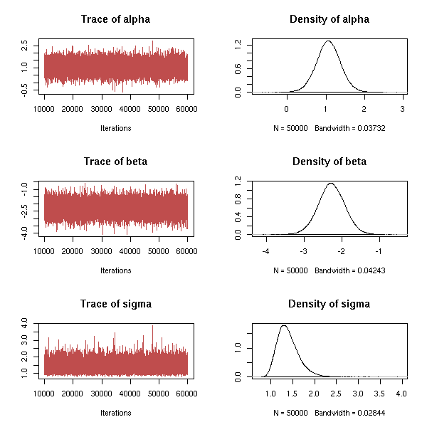
autocorr.plot(x)
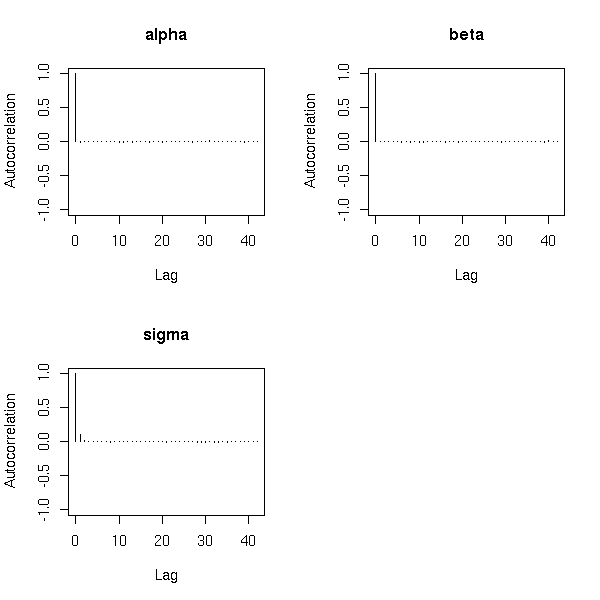
N <- 3
op <- par(mfrow=c(N,1))
for (i in 1:N) {
  pacf(x[,i], main=colnames(x)[i])
}
par(op)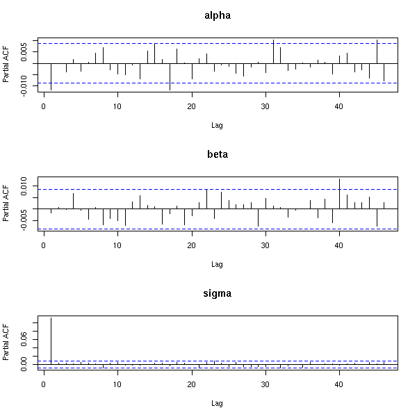
So we have a big problem for sigma: the autocorrelation is too high. The solution is to discard some values in the chain: for instance, only retain every other value, or one in ten -- or even fewer.
f <- function (x, by=2) {
  i <- seq(1, length(x), by=by)
  x[i]
}
op <- par(mfrow=c(4,1), mar=c(2,4,4,2))
for (i in 2:5) {
  pacf(f(x[,3],i), main=paste("sigma, thinning=", i, sep=""), xlab="")
}
par(op)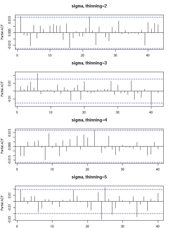
TODO: check the convergence.
> raftery.diag(x)

Quantile (q) = 0.025
Accuracy (r) = +/- 0.005
Probability (s) = 0.95

       Burn-in  Total Lower bound  Dependence
       (M)      (N)   (Nmin)       factor (I)
 alpha 2        3833  3746         1.02
 beta  2        3897  3746         1.04
 sigma 2        3833  3746         1.02
There is also a menu-driven function to assess the convergence (and other properties) of the chain(s).
codamenu()
TODO
Java program/library.
Probably easier to extend.
Slightly more difficult to use: you first have to install
Java (because of licencing issues, it cannot be as easy as
with free software), then to be able to program in Java.
Java used to be very slow, but this is no longer the case.
On the other hand, it is still very memory intensive.
The following packages will allow you to play with graphs:
graph Graph building, reading/writing GXL files Rgraphviz Plotting graphs sna Sociology ergm dynamicGraph
Examples of graphs: phylogenetic trees, citations linking research articles, metabolic pathways, interactions (regulation) between proteins and genes, social networks (friends, syringe exchanges, love affairs, phone calls, co-authoring of research papers, etc.), road traffic.
For a single problem, you can often consider several different graphs. Let us take the Web example.
1. Vertices: web pages
Edge from A to B if A contains a hyperlink to B
2. Vertices: web pages
Edge from A to B if A's URL is a prefix of B's URL
(e.g., "http://zoonek.free.fr/" is a prefix of
"http://zoonek.free.fr/foo.html")
This graph is a tree, that shows the structure of web sites.
3. Vertices: web pages
Edge between A and B if there is a document C containing
hyperlinks towards both A and B.
You can weight the edges with the number of such C documents.
4. Vertices: web pages
Edge between A and B if A and B both contain a link towards the
same document C.
Same weighting scheme as before.
5. Vertices: cartesian product {pages web} * {1,2}
Edge from (A,1) to (B,2) if A contains a hyperlink towards B.
This is a bipartite graph.Some of those graphs are oriented graphs, i.e., each edge has a direction (they are depicted as arrows), others are not (the edges are represented by segments).
A few documents that detail this:
http://www.research.att.com/%7Evolinsky/Graphs/program.html
When I try to install RGraphviz by following the instructions from the BioConductor web page, it crashes. So I install it by hand, as follows (Linux Mandrake 10.1, R-2.1.0, BioConductor 1.5).
urpmi graphviz libglib1.2-devel libgraphviz7-devel wget http://www.bioconductor.org/packages/bioc/stable/src/contrib/Source/Rgraphviz_1.5.10.tar.gz wget http://www.bioconductor.org/repository/release1.5/package/Source/Rgraphviz_1.5.0.tar.gz wget http://www.bioconductor.org/repository/release1.5/package/Source/graph_1.5.1.tar.gz wget http://www.bioconductor.org/repository/release1.5/package/Source/Ruuid_1.5.0.tar.gz wget http://www.bioconductor.org/repository/release1.5/package/Source/Biobase_1.5.0.tar.gz R CMD INSTALL Ruuid_1.5.0.tar.gz R CMD INSTALL Biobase_1.5.0.tar.gz R CMD INSTALL graph_1.5.1.tar.gz R CMD INSTALL Rgraphviz_1.5.10.tar.gz echo /usr/lib/graphviz/ >> /etc/ld.so.conf ldconfig
Sample graphs:
# One of the graphs is too large to be displayed...
library(Rgraphviz)
data(graphExamples)
op <- par(mfrow=c(6,3), mar=c(0,0,0,0))
for (g in graphExamples) {
cat(object.size(g), "\n")
if (object.size(g) < 100000) {
cat("Drawing\n")
try( plot(g) )
} else {
cat("Skipping\n")
}
}
par(op)
Some random graphs:
library(Rgraphviz)
data(graphExamples)
op <- par(mfrow=c(3,3))
set.seed(2)
for (i in 1:9) {
try( plot(randomGraph(LETTERS[1:10], 1, .3)) )
}
par(op)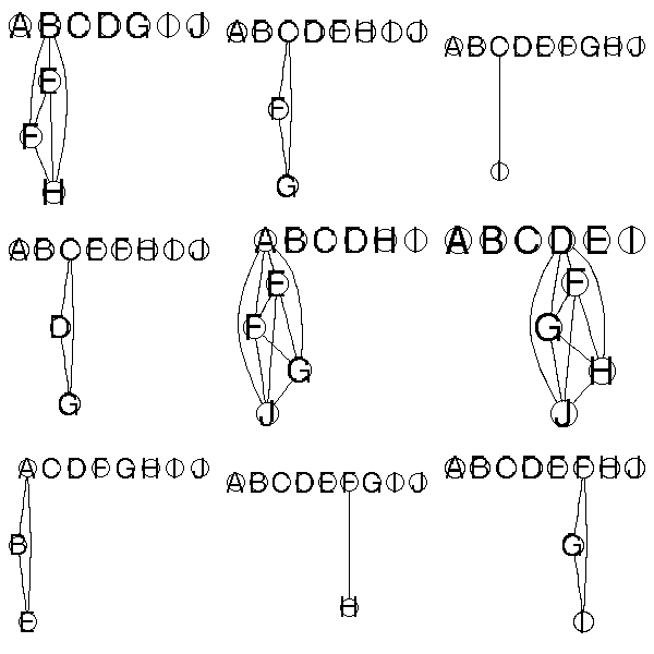
op <- par(mfrow=c(3,3))
for (i in 1:9) {
try( plot(randomGraph(LETTERS[1:10], 1, .5)) )
}
par(op)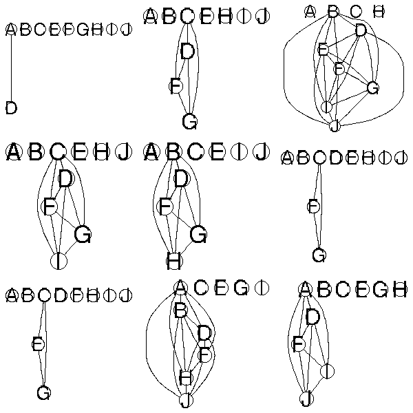
op <- par(mfrow=c(3,3))
for (i in 1:9) {
try( plot(randomGraph(LETTERS[1:10], 1, .8)) )
}
par(op)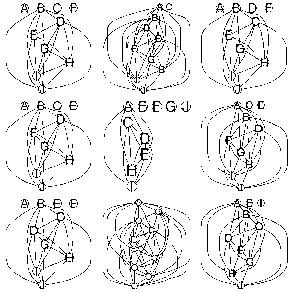
A few methods on those objects:
> g <- randomGraph(LETTERS[1:10], 1, .8)
> g
A graph with undirected edges
Number of Nodes = 10
Number of Edges = 28
> edgeMatrix(g)
A1 A2 A3 A4 A5 A6 A7 C2 C3 C4 C5 C6 C7 E3 E4 E5 E6 E7 F4 F5 F6 F7 G5 G6 G7 H6 H7 I7
from 1 1 1 1 1 1 1 3 3 3 3 3 3 5 5 5 5 5 6 6 6 6 7 7 7 8 8 9
to 3 5 6 7 8 9 10 5 6 7 8 9 10 6 7 8 9 10 7 8 9 10 8 9 10 9 10 10
> numNodes(g)
[1] 10
> isConnected(g)
[1] FALSE
> connComp(g)
[[1]]
[1] "A" "C" "E" "F" "G" "H" "I" "J"
[[2]]
[1] "B"
[[3]]
[1] "D"
> acc(g, "A")
C E F G H I J
1 1 1 1 1 1 1
> acc(g, "B")
named numeric(0)
> degree(g)
A B C D E F G H I J
7 0 7 0 7 7 7 7 7 7
> edges(g)
$A
[1] "C" "E" "F" "G" "H" "I" "J"
$B
character(0)
$C
[1] "A" "E" "F" "G" "H" "I" "J"
$D
character(0)
$E
[1] "A" "C" "F" "G" "H" "I" "J"
$F
[1] "A" "C" "E" "G" "H" "I" "J"
$G
[1] "A" "C" "E" "F" "H" "I" "J"
$H
[1] "A" "C" "E" "F" "G" "I" "J"
$I
[1] "A" "C" "E" "F" "G" "H" "J"
$J
[1] "A" "C" "E" "F" "G" "H" "I"
> complement(g)
A graph with undirected edges
Number of Nodes = 10
Number of Edges = 17Do not forget to read the documentation:
?"graph-class" ?"graphNEL-class"
The incidence matrix of such a graph:
n <- numNodes(g)
m <- matrix(0, nr=n, nc=n, dimnames=list(nodes(g),nodes(g)))
e <- edges(g)
for(i in nodes(g)) {
for (j in e[[i]]) {
m[i,j] <- 1
}
}
mConstructing a graph from its incidence matrix:
op <- par(mfrow=c(2,2))
for (a in 1:4) {
n <- 10
V <- LETTERS[1:n]
m <- matrix(sample(0:1,n*n,replace=T,prob=c(.8,.2)), nr=n, nc=n, dimnames=list(V,V))
m <- m + t(m)
m <- 1 - (m-1)*(m-2)/2
m <- m - diag(diag(m))
e <- vector("list", length=n)
names(e) <- V
for (i in 1:n) {
e[[i]] <- list( edges = which(m[i,]==1) ) # Edge numbers, not names
}
g <- new("graphNEL", nodes=V, edgeL=e)
plot(g)
}
par(op)
TODO
A random Erdos-Renyi graph is obtained as follows: choose the number of vertices and, for all vertices A and B, add an edge between A and B with probability p. One can then investigate the properties.
For graphs with many vertices, if there is, on average, less that 1 edge at each vertex, the graph will have many small connected components, if it is greater that 1, there will be a huge one containing most of the vertices.
But those graphs do not look like real-life graphs. One problem is the "clustering coefficient": it is the probability that vertices A and C be linked given that A and C are both linked to the same vertex B -- in real-world networks, it is higher. Another problem is that the distribution of the vertices valency is not poissonian.
http://arxiv.org/abs/cond-mat/0202208
library(help=corpora)

This work is licensed under a Creative Commons Attribution-NonCommercial-ShareAlike 2.5 License.
Vincent Zoonekynd
<zoonek@math.jussieu.fr>
latest modification on Sat Jan 6 10:28:26 GMT 2007