Regression with qualitative predictive variables
ANalysis Of VAriance (Anova)
ANOVA vocabulary
Mixed models
Analysis of variance is merely regression when the predictive variables are qualitative -- more precisely, it refers to the tests one performs in that context.
Covariance analysis is regression with some qualitative predictive variables and some quantitative predictive variables (the latter are then called "covariates" or "covariables").
The easiest way to understand analysis of variance is as a generalization of Student's test: it tells you if the mean of a quantitative variable is the same in several groups (Student's test is limited to the case of two groups) or, in other words, if a quantitative variables depends on a qualitative variable.
A more general way of understanding analysis of variance (and this is the point of view chosen by R's "anova" function) is as a test comparing two models: checking if a quantitative variable y depends on a qualitative variable x is equivalent to comparing the models y ~ x and y ~ 1 (if the two models are significantly different, the more complex one, y ~ x, brings more information, i.e., the quantitative variable y depends on the qualitative variable x, i.e., the mean of y is not the same in the groups defined by x).
We shall present analysis of variance in this order: regression with qualitative predictive variables, generalization of Student's test, model comparison.
In a later chapter, we shall present, more quickly, a few generalizations of analysis of variance: mixed models, hierarchical models, panel models, graphical models, bayesian networks.
TODO:
The end of this chapter is not completely written yet and
overlaps with the next chapter.
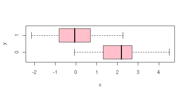
Before tackling anova itself (i.e., the tests related to a regression with qualitative predictive variables), let us focus on the regression with qualitative variables itself. Actually, there is not a big difference with classical regression.
That is simple: you code it with 0 or 1 and you perform a regression as usual.
n <- 200
x <- sample(0:1, n, replace=T)
y <- 2*(x==0) +rnorm(n)
plot( y ~ factor(x),
      horizontal = TRUE,
      xlab = 'y',
      ylab = 'x',
      col = "pink" )
plot(density(y[x==0]),
     lwd = 3,
     xlim = c(-3,5),
     ylim = c(0,.5),
     col = 'blue',
     main = "Density in each group",
     xlab = "x")
lines(density(y[x==1]),
      lwd = 3,
      col = 'red')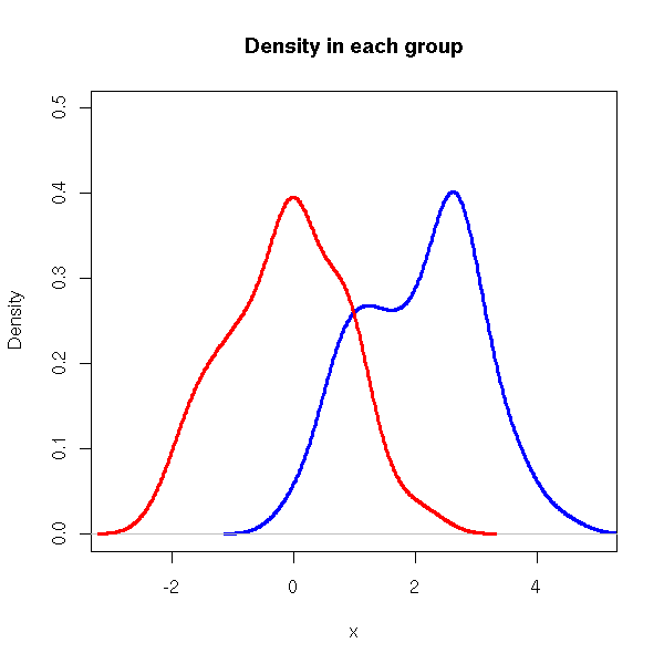
plot(y ~ x,
     main = "lm(y~x) when x is qualitative")
abline(lm(y ~ x),
       col = 'red')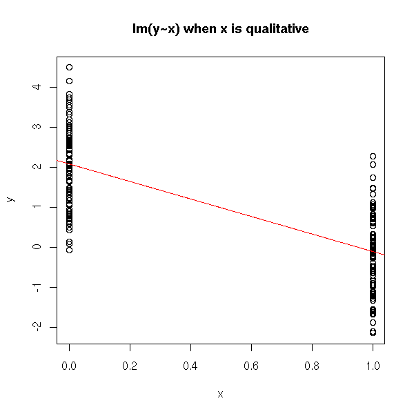
As there are only two possible values for the predictive variable, there are only two forecasts: the means of the corresponding groups.
> predict(lm(y~x), data.frame(x=c(0,1)))
         1          2
 2.0785496 -0.1654518
> tapply(y,x,mean)
       0          1
 2.0785496 -0.1654518
You can also wonder whether the means in these two groups are significantly different, with a Student test
> t.test(y[x==0], y[x==1])
      Welch Two Sample t-test
data:  y[x == 0] and y[x == 1]
t = 15.1062, df = 197.472, p-value = < 2.2e-16
or with an anova (the anova is the last line of the result ("summary") of a regression).
> summary(lm(y~x))
Call:
lm(formula = y ~ x)
Residuals:
    Min      1Q  Median      3Q     Max
-3.7520 -0.5786  0.1071  0.6504  2.7427
Coefficients:
            Estimate Std. Error t value Pr(>|t|)
(Intercept)   2.1283     0.1068   19.93   <2e-16 ***
x1           -2.1218     0.1440  -14.73   <2e-16 ***
Residual standard error: 1.013 on 198 degrees of freedom
Multiple R-Squared: 0.523,      Adjusted R-squared: 0.5206
F-statistic: 217.1 on 1 and 198 DF,  p-value: < 2.2e-16
You can also explicitely ask for an analysis of variance, i.e., explicitely compare the y ~ x model with the trivial one y ~ 1.
> anova( lm(y~x), lm(y~1) )
Analysis of Variance Table
Model 1: y ~ x
Model 2: y ~ 1
  Res.Df     RSS  Df Sum of Sq      F    Pr(>F)
1    198  203.27
2    199  426.11  -1   -222.84 217.07 < 2.2e-16 ***
I never remerber in which order to list the models to be compared: here, the number of degrees of freedom is negative, the sum of squares is negative, so the order is wrong -- but the p-value is correct. I should have put the first model first. In any case, the result is only meaningful if the models are embedded in one another, i.e., if one (the first) is a simplification of the other.
This might seem trivial: we do not need to know about regression in order to compare means -- Student's test will do. Things become less simple when you have both qualitative and quantitative variables.
We now try to predict a quantitative variable, y, from a qualitative variable, x1, and another quantitative variable, x2.
n <- 200
x1 <- sample(0:1, n, replace=T)
x2 <- rnorm(n)
y <- 1 - 2*(x1==0) + x2 +rnorm(n)
plot( y ~ x2,
      col = c(par('fg'), 'red')[1+x1],
      main = "y ~ (1 | x1) + x2")
rc <- lm( y ~ x1+x2 )$coef
abline(rc[1], rc[3])
abline(rc[1]+rc[2], rc[3],
       col = 'red')
legend(par('usr')[2], par('usr')[3], # Bottom right
       xjust = 1, yjust = 0,
       c("x1 = 0", "x1 = 1"),
       col = c("red", par("fg")),
       lty = 1,
       lwd = 3)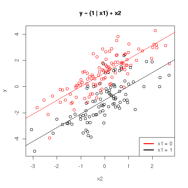
x1 <- ifelse(x1==1, "x1 = 1", "x1 = 0")
library(lattice)
xyplot( y ~ x2 | x1,
        panel = function (x, y, ...) {
          panel.xyplot(x, y, ...)
          panel.lmline(x, y)
        },
        main = "y ~ (1 | x1) + x2"
       )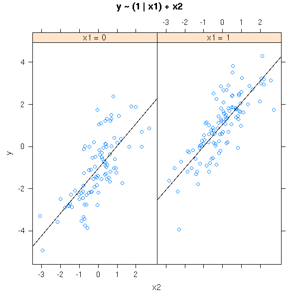
The preceding model, with no interaction term, yields parallel lines. If we add an interaction term, the lines are no longer parallel.
n <- 200
x1 <- sample(0:1, n, replace=T)
x2 <- rnorm(n)
y <- 1 + x2 - (x1==1)*(2+3*x2) + rnorm(n)
plot( y ~ x2,
      col = c(par('fg'), 'red')[1+x1],
      main = "y ~ x2 + (x2 | x1)" )
# With no interaction term (dotted lines)
rc <- lm( y ~ x1 + x2 )$coef
abline(rc[1], rc[3],
       lty = 3)
abline(rc[1]+rc[2], rc[3],
       col = 'red', lty = 3)
# with
rc <- lm( y ~ x1 + x2 + x1:x2 )$coef
abline(rc[1], rc[3])
abline(rc[1]+rc[2], rc[3]+rc[4],
       col='red')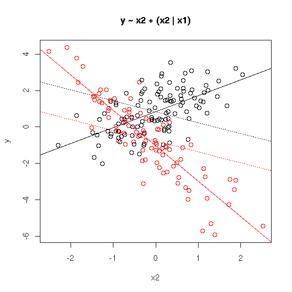
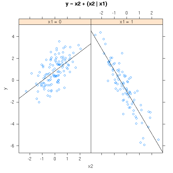
x1 <- ifelse(x1==1, "x1 = 1", "x1 = 0")
xyplot( y ~ x2 | x1,
        panel = function (x, y, ...) {
          panel.xyplot(x, y, ...)
          panel.lmline(x, y)
        },
        main = "y ~ x2 + (x2 | x1)"
       )
# One might also want to compare the intercepts
xyplot( y ~ x2 | x1,
        panel = function (x, y, ...) {
          panel.xyplot(x, y, ...)
          panel.lmline(x, y)
          panel.abline(v=0, h=0, lty=3)
        },
        main = "y ~ x2 + (x2 | x1)"
       )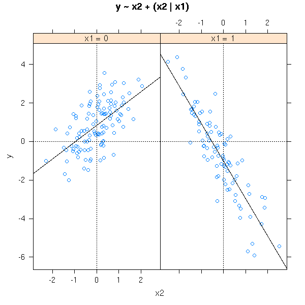
Actually, this is merely a linear regression of each value of the qualitative variable.
TODO: interaction plot (matrix plot)
if the lines are parallel, there is no interaction.
TODO
When you have several quanlitative variables, interactions can start playing an important role. For instance, it is possible that the mean of Y does not depend on X1 nor on X2, but on the pair (X1,X2). For instance
E[ Y | X=(0,0) ] > E[ Y | X=(0,1) ]
E[ Y | X=(1,0) ] < E[ Y | X=(1,1) ]
Here is a more graphical example.
n <- 1000
l <- 0:1
v <- .5
x1 <- factor( sample(l, n, replace=T), levels=l )
x2 <- factor( sample(l, n, replace=T), levels=l )
y <- ifelse( x1==0,
       ifelse( x2==0, 1+v*rnorm(n),   v*rnorm(n) ),
       ifelse( x2==0, v*rnorm(n),   1+v*rnorm(n) )
     )
boxplot( y ~ x1,
         horizontal = TRUE,
         col = "pink",
         main = "y does not seem to depend on x1",
         xlab = "y",
         ylab = "x1" )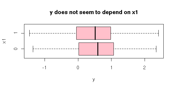
boxplot( y ~ x2,
         horizontal = TRUE,
         col = "pink",
         main = "y does not seem to depend on x2",
         xlab = "y",
         ylab = "x2" )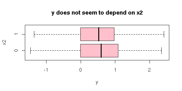
plot( as.numeric(x1) - 1 + .2*rnorm(n),
      y,
      col = c("red", "blue")[as.numeric(x2)],
      xlab = "x1 (jittered)",
      main = "Interactions between x1 and x2")
legend(par('usr')[2], par('usr')[3], # Bottom right
       xjust = 1, yjust = 0,
       c("x2 = 0", "x2 = 1"),
       col = c("red", "blue"),
       lty = 1,
       lwd = 3)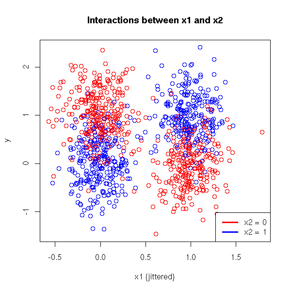
TODO: Just for fun, a 3-dimensional boxplot, with PoVRay or Rgl.
Let us consider a qualitative variable with four values: 0, 1, 2, 3.
n <- 200
x <- sample(0:3, n, replace=T)
y <- 2*(x==0) + 5*(x==2) -2*(x==3) + rnorm(n)
plot( y ~ factor(x),
      horizontal = TRUE,
      col = "pink",
      xlab = 'y',
      ylab = 'x',
      main = "x now has four values" )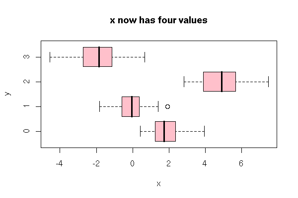
We cannot code it with those four numbers: this would imply that these values are ordered, that their effects are monotonic, that the effect of "4" is exactly twice that of "2", which is itself exactly twice that of "1". Instead, you can use several boolean variables (one also speaks of "dummy" variables, boolean variables or 0-1 variables), that assume only two values.
x1 <- as.numeric(x==1)
x2 <- as.numeric(x==2)
x3 <- as.numeric(x==3)
There are other ways of coding our qualitative variable: they will yield the same forecasts, the same statistics (F statistic, p-value, etc.), but the coefficients will have a different interpretation.
Then, we perform a regression, as usual.
> lm(y ~ x1+x2+x3)

Call:
lm(formula = y ~ x1 + x2 + x3)

Coefficients:
(Intercept)           x1           x2           x3
      2.178       -2.293        2.844       -4.110
Actually, R does this transformation itself when one of the predictive variables is a factor (beware: it HAS to be a factor, it it is merely a variable with integral values, it will be considered as a quantitative variable).
> lm(y ~ factor(x))

Call:
lm(formula = y ~ factor(x))

Coefficients:
(Intercept)   factor(x)1   factor(x)2   factor(x)3
      2.178       -2.293        2.844       -4.110
As our variable only has four values, there are only four values to predict: the means of the four groups. (You can try to interpret the coefficients direclty -- we will explain how to do that shortly -- but it is much easier, more symetric, to think in terms of predicted values.)
> predict(lm(y~factor(x)), data.frame(x=c(0,1,2,3)))
1 2 3 4
2.1778596 -0.1148520 5.0220615 -1.9325181
> tapply(y,x,mean)
0 1 2 3
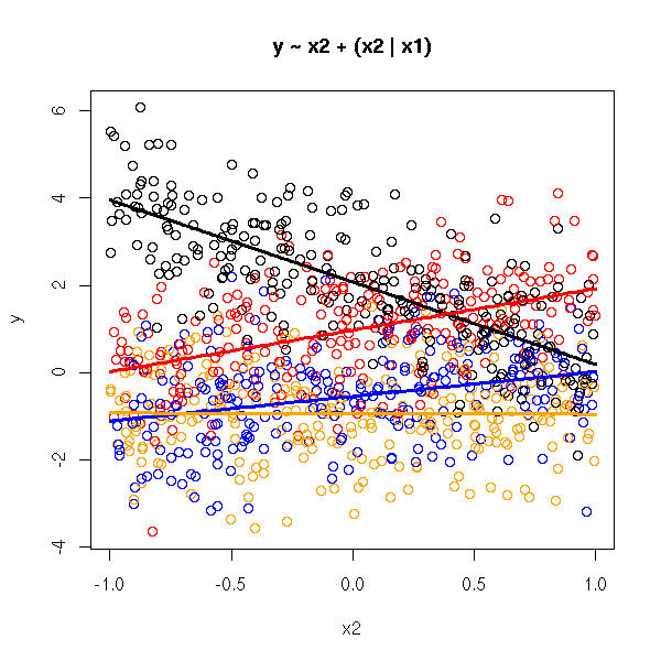
2.1778596 -0.1148520 5.0220615 -1.9325181As above, we can add in quantitative predictive variables (and here again, this is equivalent to performing a regression for each value of the qualitative variable).
n <- 1000
x1 <- sample(1:4, n, replace=T)
x2 <- runif(n, min=-1, max=1)
y <- (x1==1) * (2 - 2*x2) +
     (x1==2) * (1 + x2) +
     (x1==3) * (-.5 + .5*x2) +
     (x1==4) * (-1) +
     rnorm(n)
cols <- c(par('fg'), 'red', 'blue', 'orange')
plot( y ~ x2,
      col = cols[x1],
      main = "y ~ x2 + (x2 | x1)" )
x1 <- factor(x1)
r <- lm( y ~ x1*x2 )
xx <- seq( min(x2), max(x2), length = 100 )
for (i in levels(x1)) {
  yy <- predict(r, data.frame(
    x1 = rep(i, length(xx)),
    x2 = xx
  ))
  lines(xx, yy,
        col = cols[as.numeric(i)],
        lwd = 3)
}
If the variables are not binary, R can create the dummy variables himself. However, let us see how this can be done.
Example, with two variables:
Two qualitative variables U and V with 3 values (a, b and c).
Replace U by two variables X1 and X2.
If U=a, take X1=1 and X2=0.
If U=b, take X1=0 and X2=1.
If U=c, take X1=X2=0.
Similarly replace V by two variables X3 and X4.
The model with no interaction is
Y ~ X1 + X2 + X3 + X4
But it is not the only way of creating those dummy variables. Here is another coding.
Replace U by two variables X1 and X1
If U=a, take V1=1, V2=0.
If U=b, take V1=0, V2=1.
If U=c, take V1=V2=-1.
Similarly replace V by X3 and X4.
If you want interactions, things can become trickier...
Replace U by two variables X1 and X1
If U=a, take V1=1, V2=0.
If U=b, take V1=0, V2=1.
If U=c, take V1=V2=-1.
Similarly replace V by X3 and X4.
  Y ~ V1 + V2 + V3 + V4 + V1V3 + V1V4 + V2V3 + V2V4
You can ask R to use a coding or another.
> options()$contrasts
        unordered           ordered
"contr.treatment"      "contr.poly"

> apropos("contr\\.")
[1] "contr.helmert"   "contr.poly"      "contr.sum"       "contr.treatment"
By default, SPlus uses Helmert contrasts (but many people think it is a bad idea because they are difficult to interpret -- I personnally think they are all difficult to interpret and suggest not to interpret them directly but use them to compute quantities easier to interpret).
n <- 100
l <- 1:4
x <- factor( sample(l, n, replace=T), levels=l )
y <- ifelse(x==1, rnorm(n),
     ifelse(x==2, -4+rnorm(n),
     ifelse(x==3, -2+rnorm(n), 4+rnorm(n))))
The "model.matrix" function will tell you what matrix is actually used in the regression.
> cbind(x,y)[1:5,]
     x          y
[1,] 3 -2.1962202
[2,] 4  3.9745616
[3,] 1  0.3440235
[4,] 4  2.7521184
[5,] 2  4.3539651

> model.matrix(y~x)[1:5,]
  (Intercept) x2 x3 x4
1           1  0  1  0
2           1  0  0  1
3           1  0  0  0
4           1  0  0  1
5           1  1  0  0

> model.matrix(y~x, contrasts=list(x=contr.helmert))[1:5,]
  (Intercept) x1 x2 x3
1           1  0  2 -1
2           1  0  0  3
3           1 -1 -1 -1
4           1  0  0  3
5           1  1 -1 -1

> model.matrix(y~x, contrasts=list(x=contr.poly))[1:5,]
  (Intercept)        x.L  x.Q        x.C
1           1  0.2236068 -0.5 -0.6708204
2           1  0.6708204  0.5  0.2236068
3           1 -0.6708204  0.5 -0.2236068
4           1  0.6708204  0.5  0.2236068
5           1 -0.2236068 -0.5  0.6708204

> model.matrix(y~x, contrasts=list(x=contr.sum))[1:5,]
  (Intercept) x1 x2 x3
1           1  0  0  1
2           1 -1 -1 -1
3           1  1  0  0
4           1 -1 -1 -1
5           1  0  1  0
The default coding, "contr.treatment", is not symetric: one of the values is considered as central and the others are compared to it. You can specify which one with the "relevel" function.
Here are the results with the (default) "contr.treatment" contrasts.
> lm(y~x)

Call:
lm(formula = y ~ x)

Coefficients:
(Intercept)           x2           x3           x4
    -0.1659      -3.7780      -2.0133       3.8462
Idem with "contr.helmert".
> a <- options()$contrasts
> a[1] <- "contr.helmert"
> options(contrasts=a)
> lm(y~x)

Call:
lm(formula = y ~ x)

Coefficients:
(Intercept)           x1           x2           x3
   -0.65218     -1.88902     -0.04143      1.44416
With "contr.sum"
> a <- options()$contrasts
> a[1] <- "contr.sum"
> options(contrasts=a)
> lm(y~x)

Call:
lm(formula = y ~ x)

Coefficients:
(Intercept)           x1           x2           x3
    -0.6522       0.4863      -3.2918      -1.5270
And finally with "contr.poly".
> a <- options()$contrasts
> a[1] <- "contr.poly"
> options(contrasts=a)
> lm(y~x)

Call:
lm(formula = y ~ x)

Coefficients:
(Intercept)          x.L          x.Q          x.C
    -0.6522       2.9747       4.8188      -0.3238
Let us sum up the results.
contr.treatment   -0.1659      -3.7780      -2.0133       3.8462
contr.helmert     -0.65218     -1.88902     -0.04143      1.44416
contr.sum         -0.6522       0.4863      -3.2918      -1.5270
contr.poly        -0.6522       2.9747       4.8188      -0.3238
Let us see what happens if the effects are monotonic.
n <- 100
v <- .3
l <- 1:4
x <- factor( sample(l, n, replace=T), levels=l )
y <- ifelse(x==1, -3+v*rnorm(n),
     ifelse(x==2, -1+v*rnorm(n),
     ifelse(x==3, 1+v*rnorm(n), 3+v*rnorm(n))))
a <- options()$contrasts
for (i in c("contr.treatment", "contr.helmert", "contr.sum", "contr.poly")) {
  a[1] <- i
  options(contrasts=a)
  print(lm(y~x)$coef)
}
We get:
contr.treatment   -2.911686    1.887725    3.938457    5.914572
contr.helmert    0.02350254  0.94386256  0.99819831  0.99312780
contr.sum        0.02350254 -2.93518867 -1.04746355  1.00326881
contr.poly       0.02350254  4.42617327  0.04419473 -0.05313457
TODO: explain how to interpret the coefficients. (I am sure I have already written this somewhere...)
TODO: One could be tempted to choose another coding, easier to
interpret:
Replace U by 3 variables
If U=a, take X1=1, X2=0, X3=0
If U=b, take X1=0, X2=1, X3=0
If U=c, take X1=0, X2=0, X3=1
Explain why it does not work.
Explain how to get the corresponding coefficients.
This is another name for regression with qualitative predictive variables or, more precisely, for the tests performed in this setup.
We have seen that regression with a single qualitative predictive variable was nothing more than a computation of means. In this setup, anova is merely a test to compare means: a generalization of Student's T test, with an arbitrary number of samples (and not just two).
The assumptions are the same as with Student's T test: the samples are to be gaussian, to have the same variance, the observations are to be independant.
You can rephrase this in terms of regressions: We have two variables, X and Y, variable Y is quantitative and we are interested in its mean, variable X is qualitative (it gives the sample number, or the class of the observation -- e.g., the species if you are comparing different animal species). We want to know if Y depends in X. i.e., we perform a regression of Y against X. This can be written as
Y = a0 + a1*(X==1) + a2*(X==2) + a3*(X==3) + a4*(X==4)
and we compare this model with the trivial one
Y = b0.
Here is a simulation:
N <- 10
a <- rnorm(N)
b <- rnorm(N)
c <- rnorm(N)
d <- rnorm(N)
df <- data.frame(
  y = c(a,b,c,d),
  x = factor(c(rep(1,N), rep(2,N), rep(3,N), rep(4,N)))
)
plot( y ~ x,
      data = df,
      main = "Our 4 samples" )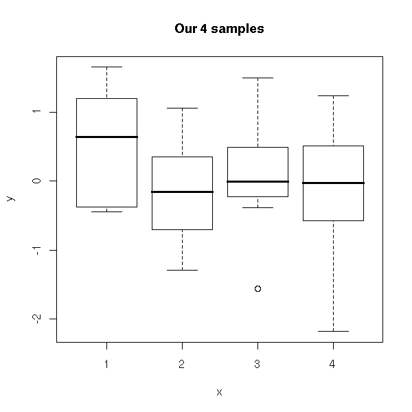
plot(density(df$y,bw=1),
     xlim = c(-6,6),
     ylim = c(0,.5),
     type = 'l',
     main = "our 4 samples",
     xlab = "y")
points(density(a,bw=1), type='l', col='red')
points(density(b,bw=1), type='l', col='green')
points(density(c,bw=1), type='l', col='blue')
points(density(d,bw=1), type='l', col='orange')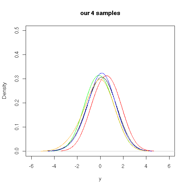
The plot below represents the value of a statistical variable on three samples. We want to know if those three samples come from the same population. To this end, we start to compare the means of those three samples. The three means will be different, of course, but will they be significantly different? Here, the difference between the means is rather high compared to the "width" of the bell-shaped curves, that have almost no overlap. For this reason, in this example, we would reject the hypothesis "the means are equal".
curve( dnorm(x-2), from=-6, to=6, col='red',
       xlab = "", ylab = "" )
curve( dnorm(x+2),    add = T, col = 'green')
curve( dnorm(x+2+.2), add = T, col = 'blue')
curve( dnorm(x+2-.3), add = T, col = 'orange')
x <- c(2, -2, -2.2, -1.7)
segments(x, c(0,0,0,0),
         x, rep(dnorm(0),4),
         col = c('red', 'green', 'blue', 'orange') )
title("The means are significantly different")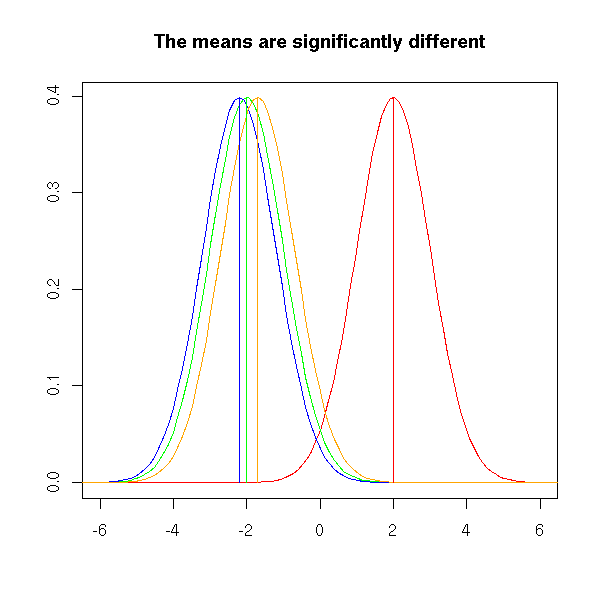
This is very different in the following plot. Even though the means are the same as above, the differences between the means are small compared to the width of the bell-shaped curves, that overlap a lot. For this reason, we shall not reject the hypothesis "the means are equal".
s <- 3
curve( dnorm(x-2, sd=s), from=-6, to=6, col='red',
       xlab = "", ylab = "" )
curve( dnorm(x+2, sd=s),    add=T, col='green')
curve( dnorm(x+2+.2, sd=s), add=T, col='blue')
curve( dnorm(x+2-.3, sd=s), add=T, col='orange')
x <- c(2, -2, -2.2, -1.7)
segments( x, c(0,0,0,0), x, rep(dnorm(0, sd=s),4),
          col=c('red', 'green', 'blue', 'orange') )
title("The means are not significantly different")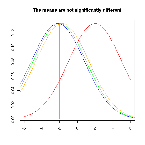
In order to quantify those qualitative and graphical reasonnings, we need a way of measuring the width of those "bell-shaped curves": we could take the variance of each sample but that would give us four numbers, one for each as we prefer a single number; so we take the mean of those variances -- if the three samples actually come from the same population, the mean of the variances is indeed an estimator of the variance of the whole population. We also need a measure of the dispersion of the means: we could take the variance of the means, but in order to compare it with the mean of the variances, we multiply it by the size of the samples -- we get another estimator of the variance of the whole population.
Finally, we consider the ratio (here, n is the size of each sample -- to simplify things, we assume they have the same size)
     n * (variance of the means)
F = -----------------------------
        mean of the variances
TODO: check this formula.
If F >> 1, we reject the hypothesis that the means are equal; if F is small, we do not reject it. As all tests, it is not symetric. One can show that if the means are equal, the the expected value of F is 1; if the means are different, the expectation is larger than 1. Of course, it happens that F<1: in that case, we do not reject the hypothesis.
This quotient, F, follows an F distribution with ******** and ****** degrees of freedom.
N <- 5000  # Iterations
n <- 5   # Sample size
k <- 3     # Number of groups
r <- rep(NA, N)
for (i in 1:N) {
  l <- matrix(rnorm(n*k), nc=k)
  r[i] <- n * var(apply(l,2,mean)) /
          mean(apply(l,2,var))
}
plot(sort(r), qf(ppoints(N),k-1,(k-1)*n),
  main = "When I know the distribution but not its parameters")
abline(0,1,col="red")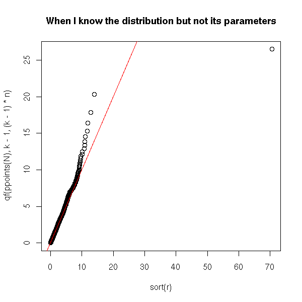
N <- 5000  # Iterations
n <- 5     # Sample size
k <- 3     # Number of groups
r <- rep(NA, N)
for (i in 1:N) {
  l <- matrix(rnorm(n*k), nc=k)
  r[i] <- n * var(apply(l,2,mean)) /
          mean(apply(l,2,var))
}
plot(sort(r), qf(ppoints(N),k-1,k*(n-1)),
  main = "When I know the distribution but not its parameters")
abline(0,1,col="red")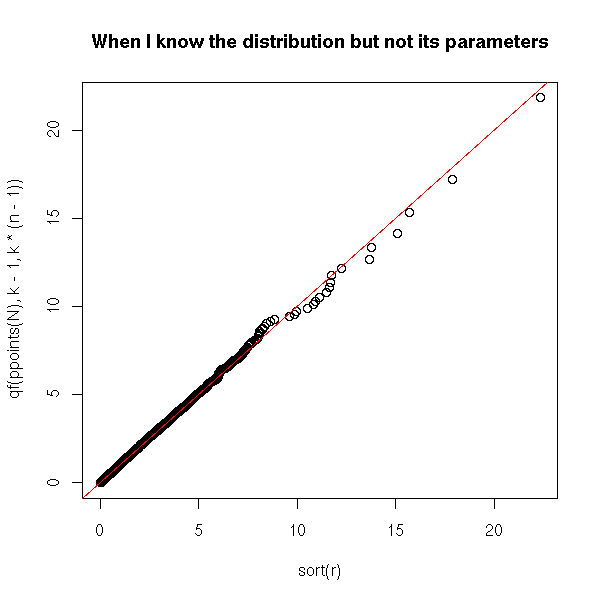
curve( df(x, 2, 2), from=0, to=4, ylim=c(0,1),
       xlab = "", ylab = "", main = "" )
curve( df(x, 2, 10), add=T, col='red' )
curve( df(x, 4, 2),  add=T, col='green' )
curve( df(x, 4, 6),  add=T, col='green' )
curve( df(x, 4, 10), add=T, col='green' )
curve( df(x, 4, 20), add=T, col='green' )
curve( df(x, 6, 2),  add=T, col='blue' )
curve( df(x, 6, 6),  add=T, col='blue' )
curve( df(x, 6, 10), add=T, col='blue' )
curve( df(x, 6, 20), add=T, col='blue' )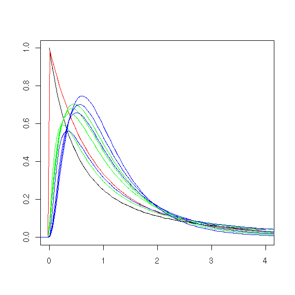
If we literally follow the definition,
n <- 10
a <- rnorm(n)
b <- rnorm(n)
c <- rnorm(n)
d <- 1+rnorm(n)
sx2 <- var(c( mean(a), mean(b), mean(c), mean(d) ))
sp2 <- mean(c( var(a), var(b), var(c), var(d) ))
MSbetween <- n * sx2
dlbetween <- 4-1
MSwithin <- sp2
dlwithin <- 4*(n-1)
F <- MSbetween / MSwithin
we find
>   F
[1] 5.137807
But usually, we perform the computations in a slightly different way, by remembering that varance may be computed from sums of squares.
Var(X) = E[ (X-EX)^2 ]
       = E[X^2] - (EX)^2
The computations then go as follows.
# Sums
sa <- sum(a)
sb <- sum(b)
sc <- sum(c)
sd <- sum(d)
s <- sa + sb + sc + sd
# Sums of squares
ssa <- sum(a^2)
ssb <- sum(b^2)
ssc <- sum(c^2)
ssd <- sum(d^2)
ss <- ssa + ssb + ssc + ssd
# The values we are interested in
# SS = Sum of Squares
# MS = Mean Square
# effect = between = explained variance
SSeffect <- (sa^2/n + sb^2/n + sc^2/n + sd^2/n) - s^2/(4*n)
dleffect <- 4-1
MSeffect <- SSeffect/dleffect
SStotal <- ss - s^2/(4*n) # ????
# error = within = residuals = residual variance
SSerror = SStotal - SSeffect
dlerror <- 4*(n-1)
MSerror <- SSerror/dlerror
F <- MSeffect / MSerror

res <- matrix( nrow=3, ncol=5 )
rownames(res) <- c("Effect", "Error", "Total")
colnames(res) <- c("SS", "df", "MS", "F", "p-value")
res[,1] <- c(SSeffect, SSerror, SStotal)
res[,2] <- c(dleffect, dlerror, dleffect+dlerror)
res[,3] <- c(MSeffect, MSerror, NA)
res[,4] <- c(F, NA, NA)
res[,5] <- c(1-pf(F,dleffect,dlerror), NA, NA)
print(res, na.print="")
This yields:
             SS df        MS        F    p-value
Effect 15.18513  3 5.0617083 5.137807 0.00463538
Error  35.46678 36 0.9851884
Total  50.65191 39
The correlation ratio is defined as
>   SSeffect/SStotal
[1] 0.2997937
We then say that "30% of the variations are explaines by the explainatory variable" (here, the "explainatory variable" is the variable telling in which group each observation is).
We now understand a little more the result produced by R:
> df <- data.frame(
+   y = c(a,b,c,d),
+   x = factor(c(rep(1,n),rep(2,n),rep(3,n),rep(4,n)))
+ )
> anova(lm(y~x, data=df))
Analysis of Variance Table

Response: y
          Df Sum Sq Mean Sq F value   Pr(>F)
x          3 15.185   5.062  5.1378 0.004635 **
Residuals 36 35.467   0.985
---
Signif. codes:  0 `***' 0.001 `**' 0.01 `*' 0.05 `.' 0.1 ` ' 1
The only number we are interested in is the p-value: here, we can reject the hypothesis "the four means are equal" with a risk of error inferior to 1%.
TODO
The model underlying analysis of variance is the following. We want to predict a quantitative variable Y with a qualitative variable X:
Y = a0 + a1*(X==1) + ... + an*(X==n) + noise
which may also be written as
Y = a_0 + a_X + noise
or (if we write i (previously X) the group of observation number j)
Y_ij = a + b_i + c_ij
The interpretation of this F test is the same as for a linear regression between quantitative variables: we measure which part of the variance of Y is explained by X.
The model may also contain several predictive variables
y  = something that depends on the value of u
     + something that depends on the value of v
     + noise
i.e.,
y = f(u) + g(v) + noise
i.e., if u and v are qualitative,
Y_ijk = a + b_i + c_j + d_ijk
We can also add some interaction terms
y  = something that depends on the value of u
     + something that depends on the value of v
     + something that depends on the value of (u,v)
     + noise
i.e.,
y = f(u) + g(v) + h(u,v)
i.e.,
Y_ijk = a + b_i + c_j + d_ij + e_ijk.
When some predictive variables are quatitative and others qualitative, we call this "covariance analysis" (and the quantitative predictive variables are called "covariates") -- but it is only a vocabulary change, the ideas, the computations are the same.
TODO: give a (real) example with two predictive variables.
In R, the "anova" command is more general: it is used to compare regression models. Analysis of variance, as we have just presented it, is actually a comparison of the model studied (say, y ~ x) with the trivial (empty) model (here, y ~ 1).
n <- 200
k <- 5
m <- sample(0:1, k, replace=T,  # The means (perhaps equal,
            p = c(.9,.1))       # perhaps not)
x <- factor(sample(1:k,n,replace=T))
y <- rnorm(n,m[x])
anova( lm(y~x), lm(y~1) )
This yields:
Analysis of Variance Table

Model 1: y ~ x
Model 2: y ~ 1
  Res.Df     RSS  Df Sum of Sq      F    Pr(>F)
1    195 184.366
2    199 226.197  -4   -41.831 11.061 4.177e-08 ***
And indeed:
> m
[1] 0 0 0 1 0
Actually, you can use the "anova" function to compare any two embedded models: for instance, two non-trivial models, or even more that two models. But the models have to be nested (to compare non-nested models, use the BIC (Bayesian Information Criterion) -- more about this somewhere else in this document).
TODO: give a real example.

anova( lm(y~x1+x2), lm(y~x1), lm(y~1) )
anova( lm(y~x1+x2), lm(y~x2), lm(y~1) )
Of course, you will be careful not to perform too many tests: each time, you have a 5% chance of claiming to see something that is not there -- in the end, you would be sure to spot some artefactual phenomenon.
TODO
One of the most disturbing things when one tries to understand analysis of variance is the vocabulary used: many complicated words, never (or rarely) explained, for very simple things. Here is a compendium of some of these words (only those I have inderstood -- and I am not even sure I have understood them properly)...
In the following examples, I shall be mainly using the "aov" function: however, I advise you not to use it unless you are absolutely confident in your understanding of its "Error" argument -- I for one, do not understand it: expect more mistakes in this part than in the rest of this document.
It is the analysis of variance with a simple predictive variable (i, in the following model).
Y_ij = a + b_i + e_ij
In R, you will write
y ~ x
where y is the variable to predict and x the predictive (qualitative) variable.
Here is an example:
n <- 30
x <- sample(LETTERS[1:3],n,replace=T, p=c(3,2,1)/6)
x <- factor(x)
y <- rnorm(n)
plot(y ~ x,
     col = 'pink',
     xlab = "", ylab = "",
     main = "Simple anova: y ~ x")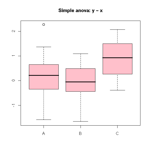
Here, the analysis of variance tells us that the three samples might have the same mean.
> summary(aov(y~x))
            Df Sum Sq Mean Sq F value Pr(>F)
x            2  2.271   1.135  1.1193 0.3307
Residuals   97 98.391   1.014
It is the analysis of variance with two predictive variables (i and j in the following model).
Y_ijk = a + b_i + c_j + e_ijk
In R, you would write
y ~ x1 + x2
In this example, the predictive variables do not interact. If you have enough data, you can look if the interact, i.e., you can compare with the model
Y_ijk = a + b_i + c_j + d_ij + e_ijk
In R, the model with an interaction term would be written
y ~ x + y + x:y
or
y ~ x * y
Here is another simulation.
n <- 100
x1 <- sample(LETTERS[1:3],n,replace=T,p=c(3,2,1)/6)
x1 <- factor(x1)
x2 <- sample(LETTERS[1:2],n,replace=T,p=c(3,1)/4)
x2 <- factor(x2)
y <- rnorm(n)
i <- which(x1=='A' & x2=='B')
y[i] <- rnorm(length(i),.5)
library(lattice)
bwplot( ~ y | x1 * x2,
       layout = c(1,6),
       main = "Double anova: y ~ x1 + x2")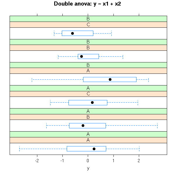
Here is the corresponding anova:
> summary(aov(y~x1*x2))
            Df Sum Sq Mean Sq F value Pr(>F)
x1           2  2.855   1.427  1.4716 0.2348
x2           1  0.487   0.487  0.5021 0.4803
x1:x2        2  0.241   0.121  0.1243 0.8833
Residuals   94 91.175   0.970
When the groups do not have the same size, the result will depend on the order in which you list the predictive variables...
> summary(aov(y~x2*x1))
            Df Sum Sq Mean Sq F value Pr(>F)
x2           1  0.798   0.798  0.8230 0.3666
x1           2  2.544   1.272  1.3112 0.2744
x2:x1        2  0.241   0.121  0.1243 0.8833
Residuals   94 91.175   0.970
In this situation you might want to use the "anova" function to compare three or four (nested) models.
anova( lm(y~1), lm(y~x1), lm(y~x1+x2), lm(y~x1*x2) )
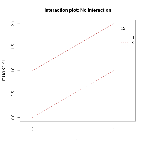
This plot can help you see if a model with two predictive variables need an interaction term.
When comparing y ~ x1 + x2 with y ~ x1 * x2, we can plot y as a function of x1, for each value of x2: we get a curve for each value of x2. You can also interchange the role of x1 and x2.
Parallel lines indicate there is no interaction.
x1 <- gl(2,2,4,c(0,1))
x2 <- gl(2,1,4,c(0,1))
n <- function (x) {
  as.numeric(as.vector(x))
}
y1 <- n(x1) + n(x2)
interaction.plot(
  x1, x2, y1,
  main = "Interaction plot: No interaction"
)
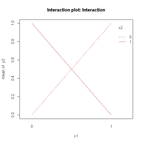
y2 <- n(x1) + n(x2) - 2*n(x1)*n(x2)
interaction.plot(
  x1, x2, y2,
  main = "Interaction plot: Interaction"
)
There are several predictive variables, say X1 and X2, and several observations for each value of (X1,X2).
This is a particular case of two-way anova -- a case in which we can, if needed, consider an interaction term: the model would be y~x1+x2 (no interaction) of y~x1*x2 (interaction).
There are several predictiva variables, say X1 and X2, and a single observation for each value of (X1,X2); in this case we do not have enough data to study the interaction between X1 and X2.
This is a particular case of two-way anova.
This is still a double anova, i.e., a model of the form
Y_ijk = a + b_i + c_j + e_ijk
but now, the value of i determines that of j, i.e., i and j both define groups in the data, and the groups defined by i are contained in those defined by j. For instance
i = Number of the leaf (from 1 to 100)
j = Number of the tree (from 1 to 10: leaves 1 to 10 are in tree 1,
                        leaves 11 to 20 on tree 2, etc.)
Other example:
i = pupil
j = classroom
Other example:
i = country
j = region (a region is a set of countries)
Here is a simulation of such data.
n <- 2000    # Number of experiments
k <- 20      # Number of subjects
l <- 4       # Number of groups
kl <- sample(1:l, k, replace=T)  # Group of each subject
x1 <- sample(1:k, n, replace=T)
x2 <- kl[x1]
A <- rnorm(1,sd=4)
B <- rnorm(k,sd=4)
C <- rnorm(l,sd=4)
y <- A + B[x1] + C[x2] + rnorm(n)
x1 <- factor(x1)
x2 <- factor(x2)
op <- par(mfrow=c(1,2))
plot(y~x1, col='pink')
plot(y~x2, col='pink')
par(op)
mtext("Hierarchical anova", line=1.5, font=2, cex=1.2)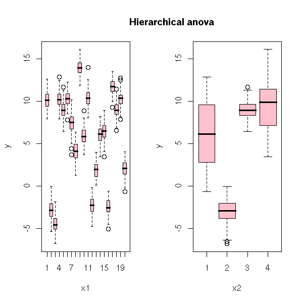
You can put this in a single plot, by using a different color for each group
# If the data were real, we wouldn't know kl.
# One may recover it that way.
kl <- tapply(x2,
             x1,
             function (x) {
               a <- table(x)
               names(a)[which(a==max(a))[1]]
             })
kl <- factor(kl, levels=levels(x2))
plot( y ~ x1, col = rainbow(l)[kl],
      main = "Hierarchical anova")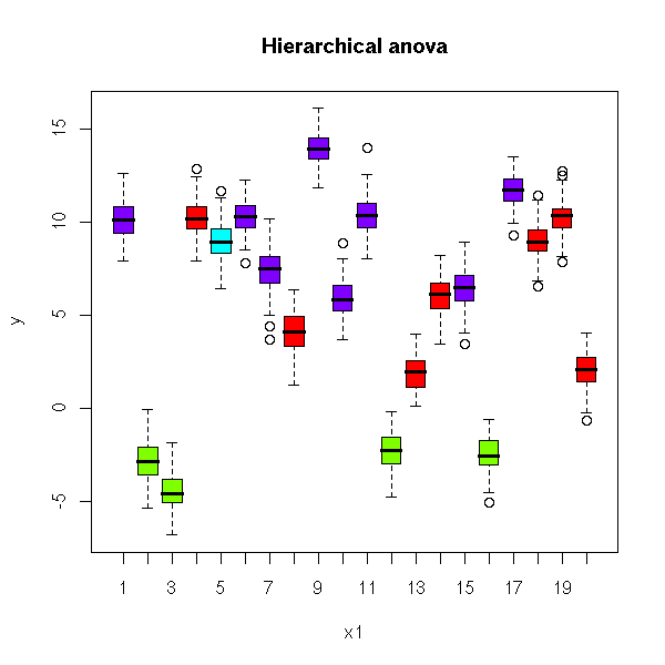
and reordering the subjects.
x1 <- factor(x1, levels=order(kl))
kl <- sort(kl)
plot( y ~ x1, col = rainbow(l)[kl],
      main = "Hierarchical anova")
legend(par('usr')[2], par('usr')[3], # Bottom right
       xjust = 1, yjust = 0,
       1:l,   # Is this right?
       col = rainbow(l),
       lty = 1,
       lwd = 3)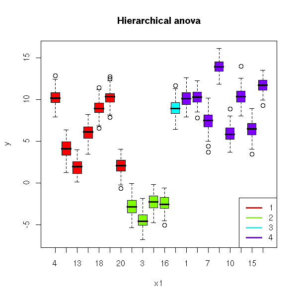
If we try to naively model this, the fact that the variables are nestes is not taken into account and prevents us from estimating the effects of x2: once we know the effects of x1, there is nothing left.
> a <- x1
> b <- x2
> lm(y~a+b)
Call:
lm(formula = y ~ a + b)
Coefficients:
(Intercept)          a11          a18          a19           a1           a2
    10.0156      -2.7380      -2.6942      -0.7015     -15.9302     -11.5106
         a8          a13          a14          a15           a3           a4
   -13.3365      -3.0425     -10.6694     -10.7422     -15.2508     -20.9595
         a9          a17          a20           a5           a7          a10
   -21.8916     -19.5307     -19.9899     -11.1213      -7.5232     -10.9528
        a12          a16           b2           b3           b4
    -5.8704      -6.5261           NA           NA           NA
Instead, we can use the "lme" function from the "nlme" package, or the "lmer" function from the newer "lme4" package.
TODO
For each subject.
For instance, we might want to compute the variance for all the observations on a given subject: this would be a "within subject" variance.
Mean (or anything else) accross all the subjects.
For instance, we can compute the variance of all the observations, regardless of the subject: this would be called the "across-subject variance".
In some cases, you can choose the values of the predictive variables, because they just describe the conditions in which the experiment was conducted.
This contrasts with the usual setup where the predictive variables are random variables.
TODO: understand what follows (actually, there are entire
books on the subject).
CRD: Completely Randomized Design
RCBD: Randomized Block Design
Latin Square: Randomized Block Design with two series of blocks
BIB: Balanced incomplete Block Design
Factorial Design
In such a design, we assume there is no difference between the subjects.
In other words, this is classical regression.
This time, we consider there are differences between the subjects. This is often the case in psychological experiments: the subjects undergo various experiments, but each subject undergoes several experiments.
You can consider the "subject" variable as another qualitative variable, whose effects should be taken into account -- but we are not _interested_ in the differences between the subjects, we do not want to know that subject 1 is faster than subject 2, but we want to account for those differences.
This is actually one motivation for the notion of mixed models.
From a practical point of view, the "anova table" in the result will have one more row, for the subjects. This is called "anova within".
We have two qualitative predictive variables, X1 and X2. We first divide the subjects into "plots", one for each value of X1. Then, in each plot, we assign each subject to a given value of X2 (i.e., we split the plot). The values of X2 are nested in those of X1. This was initially used in farming: the plots are fields (or groups of fields, close together), the subplots are sections of those fields.
We have two qualitative variables, X1 and X2, and X2 is nested within X1, i.e., X1 partitions the subjects into groups and X2 partitions each group into smaller groups. For instance:
X1: continent
X2: country

X1: (number of the) tree
X2: (number of the) leaf on the tree
A qualitative variable whose value is completely determined once we know the others. For instance, the group the subject belongs to, when each subject belongs to only one group.
See above, "in-subject design".
In an in-subject design, the tests performed on the subjects must be independant (for instance, if he is asked to perform the same task in different conditions, the second time, the differences might be due to the differing conditions or to the memory of the first experiment).
This is the name given to the parameters of the regression (i.e., the values we want to estimate).
The effects, i.e., the parameters of the regression, are numbers. This is what you are used to.
The effects, i.e., the parameters in the regression, are not numbers, but random variables, that depend on the subject.
This can be written
y = alpha + beta x + noise
alpha ~ group   # Random effect (it depends on the group)
beta ~ 1        # Fixed effect (it is the same for all the
                # observations, regardless of their group)
In this example, the intercept depends on the group, an we assume that the distribution of these intercepts is normal, with a mean and a variance to be determined, while the slope is the same for all groups. We say that the intercept is a random effect and the slope a fixed effect.
This model can also be written (this is closer to the syntax actually used by R to describe mixed models in the "lme4" package).
y ~ 1 + x + ( 1 | group )
where the terms can be read as:
1:           fixed effect (average of alpha over
             all the groups)
x:           fixed effect of x (beta, in the model above)
(1 | group): random effect (alpha, in the model above,
             has been decomposed as a sum of a
             group-independant value (fixed effect) and a
             group-dependant value (random effect) by
             requesting that the mean of the
             group-dependant value be zero).
The model is
Y_ij = a_i + b x_ij + c_ij
where
i is the subject number
j is the experiment number
x is a predictive quantitative variable
This is very similar to a classical linear regression, but the intercept depends on the subject -- the slope does not.
n <- 1000
k <- 9
subject <- factor(sample(1:k,n,replace=T), levels=1:k)
a <- rnorm(k,sd=4)
b <- rnorm(1)
x <- rnorm(n)
y <- a[subject] + b * x + rnorm(n)
plot(y~x, main="Fixed effects")
abline(lm(y~x))
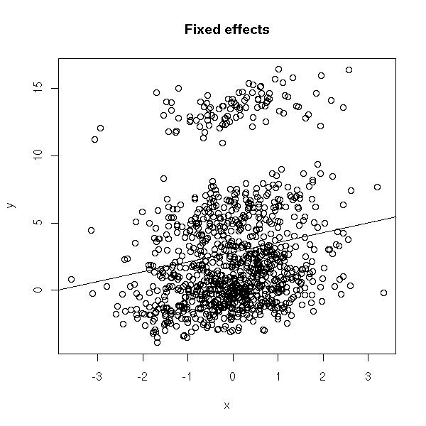
We do not see much... There is a line, indeed, but the points are very far away from this line...
Actually, there are several lines (one for each subject).
col <- rainbow(k)
plot(y~x, main="Random effects")
for (i in 1:k) {
  points(y[subject==i] ~ x[subject==i], col=col[i])
  abline( lm(y~x, subset=subject==i), col=col[i] )
}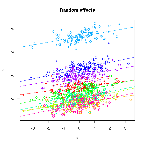
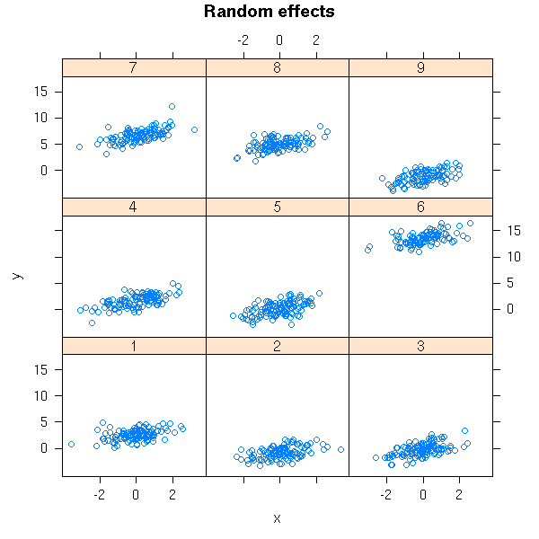
This situation is very simple: the lines are actually parallel. In real-world examples, they need not be parallel, they need not even be lines. With all the subjects on the same plot, you do not see anything -- so we use several plots.
library(lattice)
xyplot(y~x|subject, main = "Random effects")
Other name for "random effects".
The following (incomplete) table recalls the main models we have seen.
Model                                  Name
-----------------------------------------------------------------------------------
Y_ij = a + b_i + c_ij                  1-factor anova
                                       i: predictive qualitative variable

Y_ijk = a + b_i + c_j + d_ijk          2-factor anova, with no interaction
                                       i: qualitative predictive variable
                                       j: other qualitative predictive variable
                                       i and j are independant

Y_ijk = a + b_i + c_j + d_ij + e_ijk   2-factor anova, with interactions

Y_ijk = a + b_i + c_j + d_ijk          hierarchical anova
                                       i and j: predictive qualitative variables
                                       i: subject number
                                       j: group number (each subject
                                          is in only one group)
                                       j is completely determined by i
We measure the same quantity (i.e., we perform the same experiment) on each subject several times.
n <- 30
k <- 10
subject <- gl(k,n/k,n)
x <- gl(n/k,1,n)
y <- rnorm(k)
y <- rnorm(n, y[subject])
y[ x==2 ] <- y[ x==2 ] + 1

# I do not see anything
plot(y ~ x,
     col = 'pink',
     main = "Repeated measures: y ~ x | subject")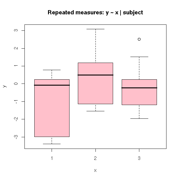
interaction.plot(
  x, subject, y,
  main = "Repeated measures: y ~ x | subject"
)
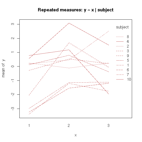
Here is the analysis of variance:
> summary(aov( y ~ x + Error(subject/x) ))

Error: subject
          Df Sum Sq Mean Sq F value Pr(>F)
Residuals  9 40.000   4.444

Error: subject:x
          Df Sum Sq Mean Sq F value   Pr(>F)
x          2 8.6491  4.3245  7.8876 0.003468 **
Residuals 18 9.8689  0.5483
Forgetting the error term is equivalent to considering the box-and-whiskers boxes above: we do not see anything.
> summary(aov(y~x))
            Df Sum Sq Mean Sq F value Pr(>F)
x            2  8.649   4.325  2.3414 0.1154
Residuals   27 49.869   1.847
We could also have taken the subject number a predictive variable: but then, we have too many parameters to estimate, there is no information (people often say "degree of freedom") left to perform a test:
> summary(aov(y~x*subject))
            Df Sum Sq Mean Sq
x            2  8.649   4.325
subject        9 40.000   4.444
x:subject     18  9.869   0.548
We shall see later that this is a "mixed model" -- no need to understand the "aov" function and its "Error" argument.
The subjects are separated into several groups and we perform several measures for each subject.
n <- 50
k <- 10
subjet <- gl(k,n/k,n)
group <- sample(1:3, k, replace=T)[subjet]
group <- factor(group)
x <- gl(n/k,1,n)
y <- rnorm(n)
y[x==1] <- y[x==1] + 1
plot(y~x, col='pink',
     main = "y ~ x | subject/group")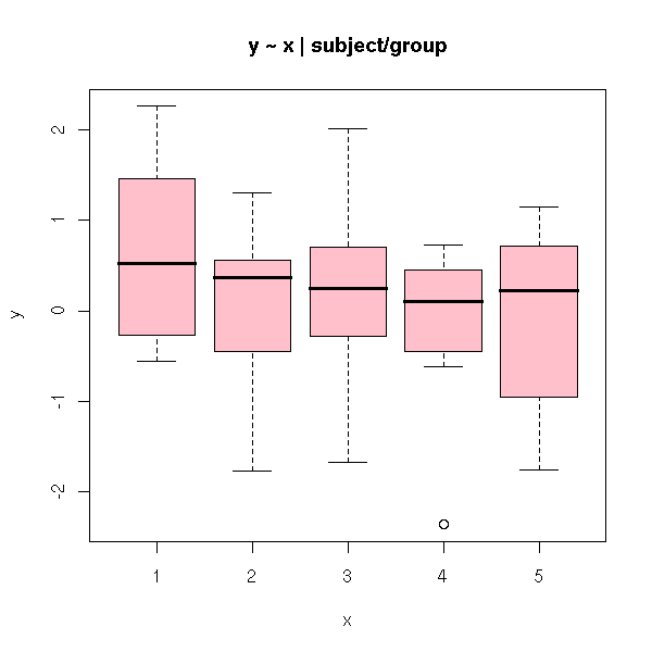
Here is the analysis of variance (x is the only within-subject factor, because each subject belongs to only one group):
> summary(aov( y ~ x * group + Error(subject/x) ))

Error: subject
          Df  Sum Sq Mean Sq F value Pr(>F)
group     2  1.7068  0.8534  0.5958 0.5768
Residuals  7 10.0260  1.4323

Error: subject:x
          Df Sum Sq Mean Sq F value  Pr(>F)
x          4 25.149   6.287  4.5296 0.00601 **
x:group   8  1.994   0.249  0.1795 0.99191
Residuals 28 38.865   1.388
This is the same as the split-splot design, but we have two levels of grouping: each subject is in a group, each group is in a class.
n <- 64
group <- gl(16,n/16,n)
supgroup <- gl(4,n/4,n)
subjet <- gl(64,n/64,n)
y <- rnorm(n)

TODO: plot
y ~ group, col=supgroup
Here, each subject appears exactly once.
The analysis of variance requires two steps: first, we check if the larger groups ("classes") are meaningful:
> summary(aov( y ~ supgroup + Error(group) ))

Error: group
          Df  Sum Sq Mean Sq F value Pr(>F)
supgroup   3  0.8376  0.2792  0.2675 0.8475
Residuals 12 12.5227  1.0436

Error: Within
          Df Sum Sq Mean Sq F value Pr(>F)
Residuals 48 50.131   1.044
then, if there are dissimilarities within the larger groups, because of the smaller groups.
> summary(aov( y ~ supgroup:group ))
                 Df Sum Sq Mean Sq F value Pr(>F)
supgroup:group   15 13.360   0.891  0.8528 0.6173
Residuals        48 50.131   1.044
TODO
Let us consider the same example, but this time, each subject appears several times.
n <- 256
group <- gl(16,n/16,n)
supgroup <- gl(4,n/4,n)
subjet <- gl(64,n/64,n)
y <- rnorm(n)
We first check if the larger groups are meaningful:
summary(aov( y ~ supgroup + Error(supgroup/group*subjet) ))

TODO: I have a few doubts
Furthermore, R takes a very long time to do the computations...
y ~ predictive variables + Error(
      Subjet / (sum or product of the predictive variables whose
                effect is likely to change from one subject to another)
    )
This allows you to perform tests:
Are there significant variations from one subject to the next?
How does the effect of the predictive variables depend on the subject?
The variables whose effects are likely to depend on the subject are sometimes called "within effects" or "within-subject factors".
The syntax
subject / v
is equivalent to
subject + v %in% subject
One-way analysis of variance: Y_ij = a + b_i + c_ij
Unbalanced anova: The groups do not have the same size
  (the computations are trickier -- but the computer does them for us)
Nested design: Y_ijk = a + b_i + c_ij + d_ijk
  No c_j term
  Example: i = tree number, j = leaf number
  Example: i = father (sire) number, j = mother number
    (in farming, the same male will be used several times, but the
     mother only once: you have to wait until she gives birth)
Nested unbalanced anova
Here is another example: we investigate the duration of a cold in subjects that have received a drug or a placebo. If we perform the experiment with different subjects, the differences between the subjects are larger that those induced by the drug.
n <- 10
subjet <- gl(n,2)
treatment <- gl(2,1,2*n, 0:1)
duration <- ifelse( treatment==1, rpois(2*n,2), rpois(2*n,3) )
summary(lm( duration ~ treatment )) # Not significant
There is no significant effect
> summary(lm( duration ~ treatment ))
Call:
lm(formula = duration ~ treatment)
Residuals:
Min 1Q Median 3Q Max
-2.20 -1.20 -0.10 0.45 3.80
Coefficients:
Estimate Std. Error t value Pr(>|t|)
(Intercept) 3.2000 0.5033 6.358 5.46e-06 ***
treatment1 -1.2000 0.7118 -1.686 0.109
---
Signif. codes: 0 `***' 0.001 `**' 0.01 `*' 0.05 `.' 0.1 ` ' 1
Residual standard error: 1.592 on 18 degrees of freedom
Multiple R-Squared: 0.1364, Adjusted R-squared: 0.08838
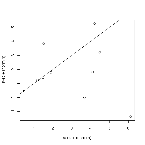
F-statistic: 2.842 on 1 and 18 DF, p-value: 0.1091However, if we perform two experiments with each subject (they have to catch two colds each), one with the placebo, one with the drug, we see that the cold is shortened by the drug.
n <- 10
subject <- gl(n,2)
traitement <- gl(2,1,2*n, 0:1)
duree <- ifelse( traitement==1, rpois(2*n,2), rpois(2*n,3) )
sans <- duree[2*(1:n)-1]
avec <- duree[2*(1:n)]
plot(sans+rnorm(n), avec+rnorm(n))
abline(0,1)
Proportion of subjects for which the drug is efficient:
> sum(sans>avec)/n
[1] 0.8
From the Wilcoxon test, it is significant
> wilcox.test(avec,sans, paired=T)

      Wilcoxon signed rank test with continuity correction

data:  avec and sans
V = 3.5, p-value = 0.02355
alternative hypothesis: true mu is not equal to 0
We can compare this with a regression.
> summary( lm(I(sans-avec) ~ 1) )

Call:
lm(formula = I(sans - avec) ~ 1)

Residuals:
   Min     1Q Median     3Q    Max
 -2.20  -0.20  -0.20   0.55   1.80

Coefficients:
            Estimate Std. Error t value Pr(>|t|)
(Intercept)   1.2000     0.3887   3.087    0.013 *
---
Signif. codes:  0 `***' 0.001 `**' 0.01 `*' 0.05 `.' 0.1 ` ' 1

Residual standard error: 1.229 on 9 degrees of freedom
Actually, this is simply a Student T test.
> t.test(sans-avec)

      One Sample t-test

data:  sans - avec
t = 3.087, df = 9, p-value = 0.01299
alternative hypothesis: true mean is not equal to 0
95 percent confidence interval:
 0.3206314 2.0793686
sample estimates:
mean of x
      1.2
You can also formulate this as a regression (it is more general: some subjects may have undergone more that two experiments).
> summary(lm( duree ~ traitement + subject )) # significant

Call:
lm(formula = duree ~ traitement + subject)

Residuals:
       Min         1Q     Median         3Q        Max
-1.100e+00 -1.750e-01  9.714e-17  1.750e-01  1.100e+00

Coefficients:
            Estimate Std. Error t value Pr(>|t|)
(Intercept)   2.6000     0.6446   4.033  0.00296 **
traitement1  -1.2000     0.3887  -3.087  0.01299 *
subject2      1.5000     0.8692   1.726  0.11849
subject3     -0.5000     0.8692  -0.575  0.57923
subject4     -1.0000     0.8692  -1.150  0.27961
subject5      2.5000     0.8692   2.876  0.01829 *
subject6      0.5000     0.8692   0.575  0.57923
subject7     -0.5000     0.8692  -0.575  0.57923
subject8      3.5000     0.8692   4.027  0.00299 **
subject9     -0.5000     0.8692  -0.575  0.57923
subject10     0.5000     0.8692   0.575  0.57923
---
Signif. codes:  0 `***' 0.001 `**' 0.01 `*' 0.05 `.' 0.1 ` ' 1

Residual standard error: 0.8692 on 9 degrees of freedom
Multiple R-Squared: 0.8712,     Adjusted R-squared: 0.7281
F-statistic: 6.088 on 10 and 9 DF,  p-value: 0.006023
We get the same value
Here is yet another way of presenting the computations:
> summary(aov(duree ~ traitement + Error(subject/traitement)))

Error: subject
          Df Sum Sq Mean Sq F value Pr(>F)
Residuals  9 38.800   4.311

Error: subject:traitement
           Df Sum Sq Mean Sq F value  Pr(>F)
traitement  1 7.2000  7.2000  9.5294 0.01299 *
Residuals   9 6.8000  0.7556
---
Signif. codes:  0 `***' 0.001 `**' 0.01 `*' 0.05 `.' 0.1 ` ' 1
However, be VERY careful at how you write those "error terms". To understand, you might want to consult
http://cran.r-project.org/doc/contrib/rpsych.html
More generally:
summary(aov( resultat ~ a1 * a2 * a3 * b1 * b2 + Error(subj/(a1+a2+a3)) ))
where a1, a2, a3 are within-subject factors and b1, b2 are between-subject factors.
 Formula              |    Model
------------------------------------------------------
 y ~ j                |    y = a_j + Error
 y ~ j + Error(i)     |    y = a_j + b_i + Error
 y ~ j + Error(i/j)   |    y = a_j + c_{i,j} + Error
Exercise: In the example above, should we writre the error term as Error(subject) or Error(subject/traitement)?
The "lme" function, in the "nlme" package, does comparable things (the data are different: otherwise, we would get a closer p-value).
> summary( lme(duree ~ traitement, random = ~ 1 | subject) )
Linear mixed-effects model fit by REML
 Data: NULL
       AIC      BIC    logLik
  67.44822 71.00971 -29.72411

Random effects:
 Formula: ~1 | subject
        (Intercept)  Residual
StdDev:   0.7601167 0.8850613

Fixed effects: duree ~ traitement
            Value Std.Error DF   t-value p-value
(Intercept)   3.2 0.3689324  9  8.673676  <.0001
traitement1  -1.3 0.3958114  9 -3.284392  0.0095
 Correlation:
            (Intr)
traitement1 -0.536

Standardized Within-Group Residuals:
        Min          Q1         Med          Q3         Max
-0.98547570 -0.73238917  0.03706879  0.48334911  1.85051895

Number of Observations: 20
Number of Groups: 10
The "nlme" function is a non-linear generalization of "lme" -- a mixture of "lme" and "nls".
Sometimes, we are not interested in all the coefficients of the model. For instance, we might want to study the effect of a drug on the results to a given test, following the model
Y_ij = a + b_i + c_j + e_ij
where i is the "treatment" variable (drug or placebo) and j is the subject number. We are interested in b_i (the effect of the drug), not in c_j (the differences between the subjects) -- however, we want to account for differences between subjects when evaluating the effects of the drug.
That is a mixed model: a regression model, when we are not interested in the actual values of some coefficients.
(There is one more difference: we shall assume that those coefficients we are interested are random variables, that follow a gaussian distribution of unknown mean and variance).
In terms of matrices, a linear model is
Y = X b + e
(X and Y anr known, we want to explain Y from X, e is random, we are looking for b) while a mixed model is
Y = X b + Z u + e
(X, Y and Z are known, u and e are random, we are looking for b). We say that b are the fixed effects and u the random effects.
These are the predictive variables we are interested in in a mixed model (more precisely, the "effects" are the corresponding coefficients).
These are the predictive variables we are not interested in. They are usually qualitative, taking a very large number of values, and we only have a few of those values (e.g., in an experiment on humans, the "subject" variable tells which human is being considered, among the 5 to 10 billions at hand -- but the experiment was only conducted on a few dozens of humans).
You might be tempted to see a mixed model as a particular case of a linear model (put X and Z in the same matrix, b and u in the same vector, estimate b and u, only report the estimated values of b). There are however a few differences.
In a mixed model, we have fewer parameters to estimate, so we can get results with fewer data.
There are also a few differences in the tests that can be performed (to use a vocabulary I do not really like: we have more "degrees of freedom" with a mixed model).
The mixed model assumes that the random effects (i.e., the coefficients we are not interested in) follow a gaussian distribution -- in a linear model, there is no such assumption.
Let us recall that in the linear model (Ordinary Least Squares, OLS), the variance of the noise term is a scalar matrix (i.e., a multiple of the identity matrix, i.e., the noise terms are independant and have the same variance). With the Generalized Least Squares, this matrix no longer need be diagonal.
This is exactly what we have in a moxed model.
Y = X b + Z u + e.
If we write R and G the variance-covariance of e and u, the variance of Y is
Var(Y) = ZGZ'+R.
So, even if e and u are scalar matrices, the variance of Y can be more complex: the moxed model is not a particular case of the linear model where we discard the coefficients we are not interested in, but rather a particular cas of generalized least squares.
The following terms are more or less equivalent:
Mixed models
Random Coefficient Model

HLM (Hierarchical Level Model)
Multilevel Analysis
Grouped Data

Panel Data
Longitudinal Data
In classical models, we have a universe (for instance, the British population) from which we sample subjects, at random, in which we perform experiments or measurements (income, sex, age, weight, etc.).
In hierarchical model, this sampling is performed in (at least) two steps. We have a first universe (say, that of British cities), from which we sample. For each of those elements, we measure a few variables of interest (latitude, longitude, size, taxes, average income, etc.). For each of those elements (cities), we have another universe (its inhabitants), from which we now sample elements (people) on which we measure the variables we are interested in (income, age, etc.)
If we out the collected data in a table, we get two tables.
City          Area           Inhabitants
----------------------------------------
A                1                 28000
B                7                 50000
C                3                 15000

Subject  City       Income  Age
-------------------------------
Artaud      A           30   32
Balzac      A           50   38
Camus       B           10   21
Descartes   C           20   49
Etiemble    C           27   36
Fenelon     C           23   29
Gide        B           15   56
It will be easier to put everything in a single table -- but some data will be repeated.
Subject  City            Area         Inhabitants   Income  Age
---------------------------------------------------------------
Artaud      A               1               28000       30   32
Balzac      A               1               28000       50   38
Camus       B               7               50000       10   21
Descartes   C               3               15000       20   49
Etiemble    C               3               15000       27   36
Fenelon     C               3               15000       23   29
Gide        B               7               50000       15   56
In this example, we have two sampling levels (city and subject) and we have variables defined at each level (area and number of inhabitants are defined for the cities, i.e., are the same for all the inhabitants of a given city; income and age are subject-level variables).
Now that we have given a numeric example, let us perform a few simulations and look at a few plots.
# There are 12 cities
n.cities <- 12

# The area of those cities (more reasonably, the logarithm
# of their areas) are gaussian, independant variables.
area.moyenne <- 5
area.sd <- 1
area <- rnorm(n.cities, area.moyenne, area.sd)

a <- rnorm(n.cities)
b <- rnorm(n.cities)

# 200 inhabitants sampled in each city
n.inhabitants <- 20
city <- rep(1:n.cities, each=n.inhabitants)

# The age are independant gaussian variables, mean=40, sd=10
# We could have chosen a different distribution for each city.
# (either randomly, or depending on their area or population).

age <- rnorm(n.cities*n.inhabitants, 40, 10)

# The income (the variable we try to explain) is a function of the
# age, but the coefficients depend on the city
# Here, the coefficients are taken at random, but they could
# depend on the city area or population.
# Here, the coefficients are independant -- this is rarely the case
a <- rnorm(n.cities, 20000, sd=2000)
b <- rnorm(n.cities, sd=20)
income <- 200*area[city] + a[city] + b[city]*age +
          rnorm(n.cities*n.inhabitants, sd=200)

plot(income ~ age, col=rainbow(n.cities)[city], pch=16)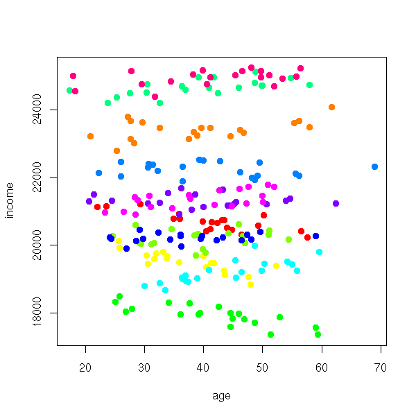
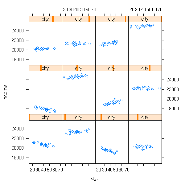
We do not see much on this plot. One idea is to consider a different plot for each city: this is what the "lattice" package provides (recall that the general idea of "lattice" (or "treillis") plots: slicing a cloud of points). Remember the syntax,
variable to predict ~ predictive variables | group
we shall use it again when estimating the coefficients of mixed models (i.e., estimating the mean and variance of a and b, the covariance of (a,b), performing tests to know if a and b really depend on the city).
library(lattice)
xyplot(income ~ age | city)
In this example, both a and b depended on the city. But perhaps only one of them depends n the city -- or even, none.
a <- rnorm(n.cities, 20000, sd=2000)
b <- rep(rnorm(1, sd=20), n.cities)
income <- 200*area[city] + a[city] + b[city]*age +
          rnorm(n.cities*n.inhabitants, sd=200)
xyplot(income ~ age | city)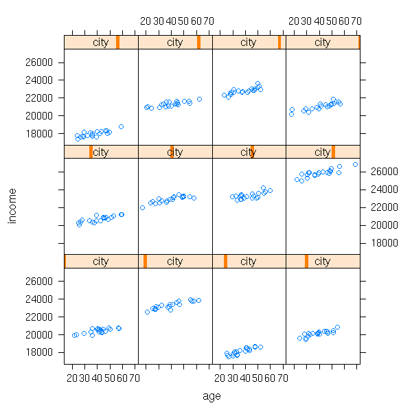
a <- rep( rnorm(1, 20000, sd=2000), n.cities )
b <- rnorm(n.cities, sd=20)
income <- 200*area[city] + a[city] + b[city]*age +
          rnorm(n.cities*n.inhabitants, sd=200)
xyplot(income ~ age | city)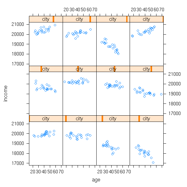
a <- rep( rnorm(1, 20000, sd=2000), n.cities )
b <- rep(rnorm(1, sd=20), n.cities)
income <- 200*area[city] + a[city] + b[city]*age +
          rnorm(n.cities*n.inhabitants, sd=200)
xyplot(income ~ age | city)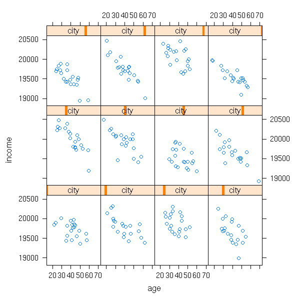
Mixed models appear when the observations are no longer independant: the subjects belong to groups (we know the groups, but there are too many of them, we cannot take a subject from all the groups) and the variables measured on the subjects of a given group have similar values.
TODO: more details
TODO: give an example?

Example: The results at an exam depend on the class.
Example: cluster sampling
You can have more that two levels:
student/class/teacher/school/city/country

TODO: other examples
You can move the variables from one level to another: for instance, you can consider the income of a subject, or the average income in a city.
TODO: give the R syntax to describe those more complicated models.
The various random variables at hand need not be independant: the model can give the shape of this variance-covariance matrix.
TODO: details
TODO: more precise examples
A commom mistake is to perform an analysis at a given level and draw conclusitons at another.
Example: if there is a correlation between the rate of illiteracy and the presence of a certain ethnic minority, this does not mean that you will have the same correlation at the subject level.
But rest reassured, you can of course perform multi-level analyses, for instance, by trying to predict a subject-level variable from subject-level and group-level variables.
For instance, the name of the city should not be used to predict anything -- simply because we have sampled among the cities, we do not have all the cities.
The first idea (and often, the first step), when analysing grouped data, is to perform a regression in each group (or, at least, look at each group separately -- e.g., with a lattice plot). Let us go back to one of our simulated examples above.
n.cities <- 12
area <- rnorm(n.cities, 5, 1)
a <- rnorm(n.cities)
b <- rnorm(n.cities)
n.inhabitants <- 20
city <- rep(1:n.cities, each=n.inhabitants)
age <- rnorm(n.cities*n.inhabitants, 40, 10)
a <- rnorm(n.cities, 20000, sd=2000)
b <- rep(rnorm(1, sd=20), n.cities)
income <- 200*area[city] + a[city] + b[city]*age +
rnorm(n.cities*n.inhabitants, sd=200)
xyplot(income ~ age | city)
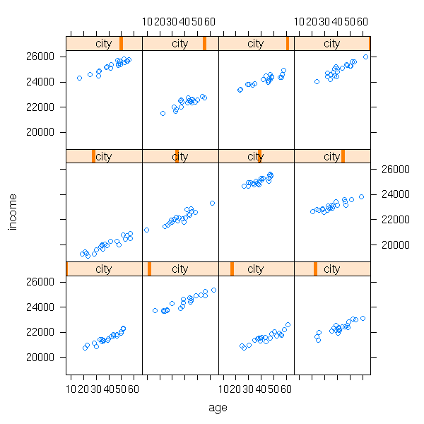
The "lmList" function in the "nlme" package performs a regression in each group.
library(nlme)
d <- data.frame(income, age, city, area=area[city])
r <- lmList(income ~ age | city, data=d)
this yields:
> summary(r)
Call:
  Model: income ~ age | city
   Data: d

Coefficients:

   (Intercept)
   Estimate Std. Error   t value Pr(>|t|)
1  21479.14   162.7878 131.94565        0
2  24026.24   274.6432  87.48163        0
3  19633.32   169.5408 115.80292        0
4  17354.47   205.3334  84.51853        0
5  22675.63   207.5127 109.27345        0
6  22732.46   235.9244  96.35486        0
7  21292.20   178.5410 119.25666        0
8  20044.50   185.1989 108.23230        0
9  18924.25   136.4418 138.69835        0
10 20630.17   147.8031 139.57873        0
11 20572.80   170.0011 121.01566        0
12 18025.29   180.2910  99.97887        0

   age
     Estimate Std. Error     t value   Pr(>|t|)
1  -6.0190190   4.343643 -1.38570746 0.16726531
2   4.3642466   6.469611  0.67457638 0.50066630
3   5.1117531   4.252501  1.20205817 0.23065717
4   0.2409800   5.088937  0.04735370 0.96227508
5   0.2023943   5.150521  0.03929589 0.96869078
6   8.0885149   5.755782  1.40528515 0.16137312
7   7.9947740   4.245020  1.88333011 0.06099939
8   4.2547386   4.528523  0.93954232 0.34850184
9   2.9008258   3.713258  0.78120777 0.43553568
10  3.4318408   3.813179  0.89999457 0.36912542
11 -3.1825003   3.956591 -0.80435410 0.42207690
12 -1.3094108   4.573603 -0.28629742 0.77492474

Residual standard error: 195.6667 on 216 degrees of freedom
Here, we see that the intercept depends on the city while the slope does not. We say that the intercept is a "random coefficient" (or a random effect) and that the slope is a fixed coefficient (or a fixed effect).
library(nlme)
d <- data.frame(income, age, city, area=area[city])
r <- lmList(income ~ age | city, data=d)
plot(intervals(r))
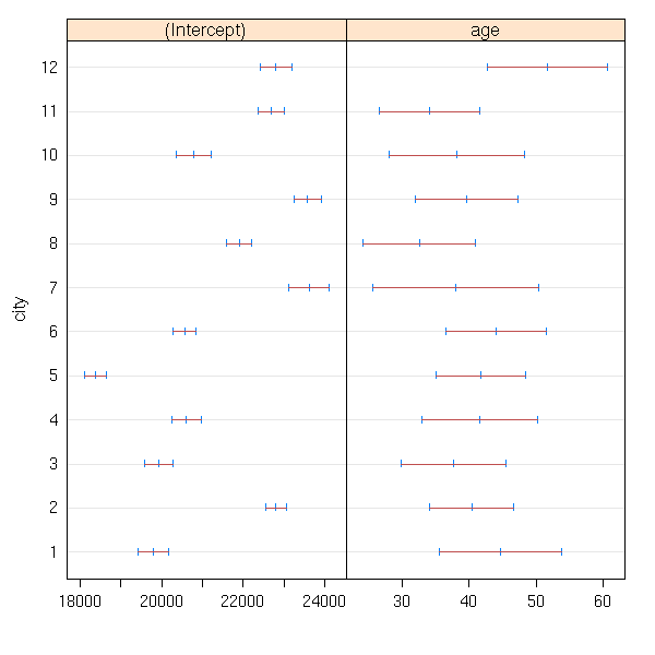
Exercise: Take the area into account.
The rest...

This work is licensed under a Creative Commons Attribution-NonCommercial-ShareAlike 2.5 License.
Vincent Zoonekynd
<zoonek@math.jussieu.fr>
latest modification on Sat Jan 6 10:28:23 GMT 2007