Example: a classification problem
Naive Bayes classifyer
Discriminant Analysis
Logistic Regression
TODO
Variants of logistic regression
Let us now tackle regression when the variable to predict is qualitative.
TODO: In this chapter, I mention Discriminant Analysis, already tackled in the chapter about PCA. Choose where to detail this...
TODO: Include LDA, naive bayesian classifier
For the moment, in the regressions we have seen, the variable to predict was always a (continuous) quantitative variable. However, this already enables us to investigate some situations in which qualitative variables appear. Here is an example.
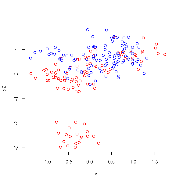
We have three variables, two of them quantitative, X1 and X2, and one qualitative Y, with two values. We want to predict Y from X1 and X2.
n <- 10
N <- 10
s <- .3
m1 <- rnorm(n, c(0,0))
a <- rnorm(2*N*n, m1, sd=s)
m2 <- rnorm(n, c(1,1))
b <- rnorm(2*N*n, m2, sd=s)
x1 <- c( a[2*(1:(N*n))], b[2*(1:(N*n))] )
x2 <- c( a[2*(1:(N*n))-1], b[2*(1:(N*n))-1] )
y <- c(rep(0,N*n), rep(1,N*n))
plot( x1, x2, col=c('red','blue')[1+y] )
We can consider the qualitative variable as a quantitative variable, assuming two values, 0 and 1, and perform a linear regression against the others. We get an expression of the form
Y = b0 + b1 X1 + x2 X2.
We can then part the (X1,X2) plane in two, along the "b0 + b1 X1 + x2 X2 = 1/2" line.
plot( x1, x2, col=c('red','blue')[1+y] )
r <- lm(y~x1+x2)
abline( (.5-coef(r)[1])/coef(r)[3], -coef(r)[2]/coef(r)[3] )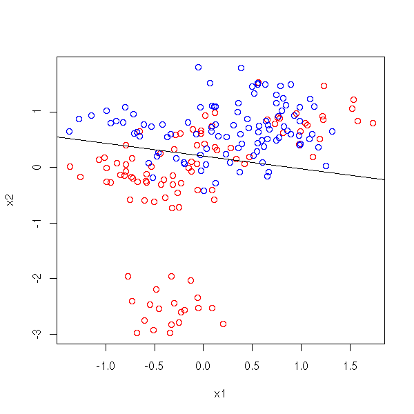
The situation is the same as above, but this time, we regress Y against X1, X2, X1X2, X1^2, X2^2.
# I need a function to draw conics...
conic.plot <- function (a,b,c,d,e,f, xlim=c(-2,2), ylim=c(-2,2), n=20, ...) {
  x0 <- seq(xlim[1], xlim[2], length=n)
  y0 <- seq(ylim[1], ylim[2], length=n)
  x <- matrix( x0, nr=n, nc=n )
  y <- matrix( y0, nr=n, nc=n, byrow=T )
  z <- a*x^2 + b*x*y + c*y^2 + d*x + e*y + f
  contour(x0,y0,z, nlevels=1, levels=0, drawlabels=F, ...)
}
r <- lm(y~x1+x2+I(x1^2)+I(x1*x2)+I(x2^2))$coef
plot( x1, x2, col=c('red','blue')[1+y] )
conic.plot(r[4], r[5], r[6], r[2], r[3], r[1]-.5,
           xlim=par('usr')[1:2], ylim=par('usr')[3:4], add=T)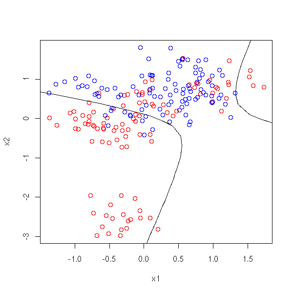
The situation is still the same. This time, in order to find the value of Y from those of X1 and X2, we take the 10 points of the sample nearest from (X1,X2), we average the corresponding Y values and round to 0 or 1.
M <- 100
d <- function (a,b, N=10) {
  mean( y[ order( (x1-a)^2 + (x2-b)^2 )[1:N] ] )
}
myOuter <- function (x,y,f) {
  r <- matrix(nrow=length(x), ncol=length(y))
  for (i in 1:length(x)) {
    for (j in 1:length(y)) {
      r[i,j] <- f(x[i],y[j])
    }
  }
  r
}
cx1 <- seq(from=min(x1), to=max(x1), length=M)
cx2 <- seq(from=min(x2), to=max(x2), length=M)
plot( x1, x2, col=c('red','blue')[1+y] )
contour(cx1, cx2, myOuter(cx1,cx2,d), levels=.5, add=T)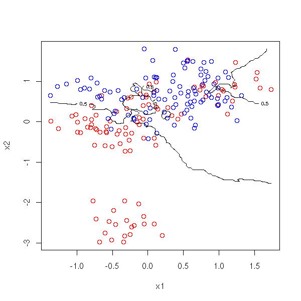
The problem of the "outer" function is mentionned in the FAQ, where they provide another solution, more "parallelized" than mine...
wrapper <- function(x, y, my.fun, ...) {
  sapply(seq(along=x), FUN = function(i) my.fun(x[i], y[i], ...))
}
outer(cx1,cx2, FUN = wrapper, my.fun = d)
Here is another situation in which the nearest neighbours method proves more relevant than the preceding.
n <- 20
N <- 10
s <- .1
m1 <- rnorm(n, c(0,0))
a <- rnorm(2*N*n, m1, sd=s)
m2 <- rnorm(n, c(0,0))
b <- rnorm(2*N*n, m2, sd=s)
x1 <- c( a[2*(1:(N*n))], b[2*(1:(N*n))] )
x2 <- c( a[2*(1:(N*n))-1], b[2*(1:(N*n))-1] )
y <- c(rep(0,N*n), rep(1,N*n))
plot( x1, x2, col=c('red','blue')[1+y] )
M <- 100
cx1 <- seq(from=min(x1), to=max(x1), length=M)
cx2 <- seq(from=min(x2), to=max(x2), length=M)
#text(outer(cx1,rep(1,length(cx2))),
#     outer(rep(1,length(cx1)), cx2),
#     as.character(myOuter(cx1,cx2,d)))
contour(cx1, cx2, myOuter(cx1,cx2,d), levels=.5, add=T)
# Color the various areas
points(matrix(cx1, nr=M, nc=M),
       matrix(cx2, nr=M, nc=M, byrow=T),
       pch='.',
       col=c("red", "blue")[ as.numeric( myOuter(cx1,cx2,d) >.5 )+1])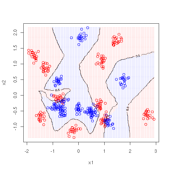
pastel <- .9
plot( x1, x2, col=c('red','blue')[1+y] )
points(matrix(cx1, nr=M, nc=M),
       matrix(cx2, nr=M, nc=M, byrow=T),
       pch=16,
       col=c(rgb(1,pastel,pastel), rgb(pastel,pastel,1))
           [ as.numeric( myOuter(cx1,cx2,d) >.5 )+1])
points(x1, x2, col=c('red','blue')[1+y] )
contour(cx1, cx2, myOuter(cx1,cx2,d), levels=.5, add=T)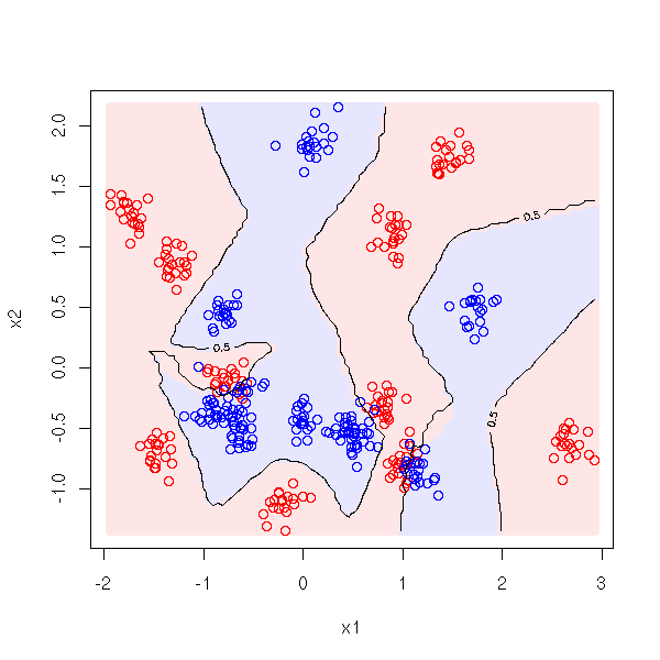
Let us vary the number of neighbours.
plot( x1, x2, col=c('red','blue')[1+y] )
v <- c(3,10,50)
for (i in 1:length(v)) {
  contour(cx1, cx2,
          myOuter(cx1,cx2, function(a,b){d(a,b,v[i])}),
          levels=.5, add=T, drawlabels=F, col=i+1)
}
legend(min(x1),max(x2),as.character(v),col=1+(1:length(v)), lty=1)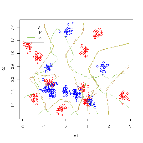
We remark that we should not take too many points.
If we do not take the 10 nearest points but just the nearest point, we get a Voronoi diagram.
http://www.perlmonks.org/index.pl?node_id=189941

Here is a funny application of Voronoi tessellations: sea ice
modeling in computer-generated images (you can reuse the idea for
giraffe skin):

http://images.povcomp.com/entries/images/210_detail2.jpg
http://www.povcomp.com/entries/210_detail2.php
http://www.povcomp.com/entries/210.php
http://trific.ath.cx/software/gimp-plugins/voronoi/
They are also used to create mosaics.
http://nis-ei.eng.hokudai.ac.jp/~doba/papers/egshort02_mosaic.pdf

We shall see another application of Voronoi diagrams to spot
outliers.
TODO
Other applications:
http://www.voronoi.com/cgi-bin/voronoi_applications.php

TODO: give more examples...
There are several variants of this method: instead of taking the mean on the 10 neighbours, we can take all the points but weigh them according to the distance to our point (such a weighting scheme is called a "kernel"); we can replace the euclidian distance by another, more relevant to the data; etc.
Given a set of points x1, x2, ..., xN in R^n, and a new point y, we want to finc the x_i nearest to y. The naive method consists in examining all the points in turn, compute their distance with y, and retain the nearest. This may be fine of there is a single new point y, but it is not very efficient if we plan to use it on many new points. Instead, we can preprocess the points x1, ..., xN so as to quickly find the one nearest to a new given point.
In dimension one, this can be done as follows; instead of representing the points as an unordered cloud, represent them as a tree: find the median, cut the cloud of points in two along the median, proceed recursively with thowe two new clouds.
TODO: give an example.
(a numeric example; plot the tree, give a 1-dimensional
plot as we shall shortly be doing in 2 dimensions)
This is used to speed up data access in a database (when you create an "index" on a numeric variable); it works well for requests of the form
Find the records for which x = 17
Find the records for which x <= 9
Find the records for which 9 <= x and x <= 17
This can be generalized in higher dimensions, under the name "kD tree" (for "k-dimensional tree"): we split the cloud of points along the median of one of the coordinates and we change the coordinate used at each step.
TODO: plot in 2D
There are several ways of choosing which coordinate to use for the split, e.g., "take each coordinate in turn, cyclically"; or "median of the most spread dimension"; or (instead of the median) "the point closest to the center of the widest dimension" (this enforces more square cells).
TODO: plots, for those three algorithms, in two examples:
uniform random points in a square
points along a circle (this tends to be pathological).
As in dimension 1, this is used in DBMS (DataBase Management Systems) to speed up requests of the form
Find the records with x = 17, y = 3 and z = 5
Find the records with x = 17
Find the records with x <= 17
For the last two examples, we explore the tree, but when it forks according to y or z, we have to explore both branches.
TODO: a plot of such a tree?
kD trees can also be used to find the nearest neighbour of a point: the idea is to proceed as with the naive algorithm, by examining all the points, but instead of takeing them in an arbitrary order, we follow the tree ("depth first") and we remember to distance to the closedt point found so far: this allows us to prune whole branches, if their points are farther that our best guess so far.
The main applications of k-D trees (and their generalization, BSP (Binary Space Partitionning) trees, where the cutting hyperplanes need not be orthogonal to the axes) are: indexing geographical data (in spacial dsatabases or GIS, Geographical Information Systems); indexing multidimensional data in databases, even if the data are not geographical; culling objects from 3-dimensional scenes, i.e., quickly deciding what is visible and should be rendered and what is not currently visible and can thus be safely discarded; description of FPS (First Person Shooter) video game levels (e.g., Quake); local regression, i.e., regression on the k nearest neighbours of each point of our sample (contrary to the naive implementation, that precomputes the regression at each sample point, kD trees allow us to perform the computations on the fly and therefore allow you to change the parameters (kernel width, degree) without needing a retraining phase -- the training phase basically consists in storing the data); reducing the number of colours in an image (represent the colours as points in the 3-dimensional red-green-blue space, build a kD-tree on those points, stop when you have the desired number of leaves, replace each leaf by its median); simulating the n-body problem (build the kD tree of the n objects, for each node (starting with the deepest nodes), compute the forces between its children (considered as points)).
http://www.autonlab.org/autonweb/documents/papers/moore-tutorial.pdf
http://en.wikipedia.org/wiki/Binary_space_partitioning
http://en.wikipedia.org/wiki/Doom_engine
http://groups.csail.mit.edu/graphics/classes/6.838/S98/meetings/m13/kd.html
http://www.cs.cmu.edu/~kdeng/thesis/kdtree.pdf
http://www.liacc.up.pt/~ltorgo/PhD/th5.pdf
http://www.flipcode.com/articles/article_raytrace07.shtml
Regression is much more stable, it works fine with few observations, but the results are imprecise. Furthermore, it assumes that the data have a simple structure.
On the contrary, the nearest neighbour method is more precise, does not assume anything about the structure of the data, but is not very stable (i.e., a different sample can yield completely different results) and works best with many observations.
Furthermore, the nearest neighbour method falls under the curse of dimension: if the dimension is high, the "nearest" neighbours are far away, most points are approximately at the same distance from our point...
TODO: take two samples, a small (100 or 200 observations, to do the computations, and another, larger (1e4), to validate them. Plot the error rate as a function of the number of neighbours. TODO: check that it works...
get.model <- function (n=10, m=2, s=.1) {
  list( n=n, m=m, x=runif(n), y=runif(n), z=sample(1:m,n,replace=T), s=s )
}
get.sample <- function (model, n=200) {
  i <- sample( 1:model$n, n, replace=T )
  data.frame( x=rnorm(n, model$x[i], model$s),
              y=rnorm(n, model$y[i], model$s),
              z=model$z[i] )
}
nearest.neighbour.predict <- function (x, y, d, k=10) {
  o <- order( (d$x-x)^2 + (d$y-y)^2 )[1:k]
  s <- apply(outer(d[o,]$z, 1:max(d$z), '=='), 2, sum)
  order(s, decreasing=T)[1]
}
m <- get.model()
d <- get.sample(m)
N <- 1000
d.test <- get.sample(m,N)
n <- 50
r <- rep(0, n)
# Very slow
for (k in 1:n) {
  for(i in 1:N) {
    r[k] <- r[k] +
      (nearest.neighbour.predict(d.test$x[i], d.test$y[i], d, k) != d.test$z[i] )
  }
}
plot(r/N, ylim=c(0,1), type='l', xlab="Error rate")
abline(h=c(0,.5,1), lty=3)
rm(d.test)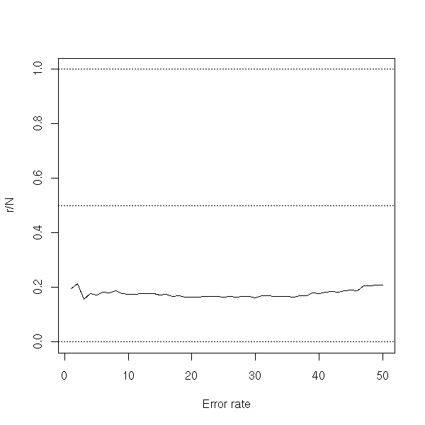
With a smaller sample:
m <- get.model()
d <- get.sample(m, 20)
N <- 1000
d.test <- get.sample(m,N)
n <- 50
r <- rep(0, n)
# Very slow
for (k in 1:n) {
  for(i in 1:N) {
    r[k] <- r[k] +
      (nearest.neighbour.predict(d.test$x[i], d.test$y[i], d, k) != d.test$z[i] )
  }
}
plot(r/N, ylim=c(0,1), type='l', xlab="Error rate")
abline(h=c(0,.5,1), lty=3)
rm(d.test)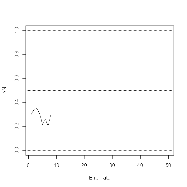
The nearest neighbour method remains valid with more than two classes.
nearest.neighbour.plot <- function (d, k=10, model=NULL) {
  col <- rainbow(max(d$z))
  plot( d$x, d$y, col=col )
  cx <- seq(min(d$x), max(d$x), length=100)
  cy <- seq(min(d$y), max(d$y), length=100)
  pastel <- .8
  colp <- round(pastel*255 + (1-pastel)*col2rgb(col))
  colp <- rgb(colp[1,], colp[2,], colp[3,], max=255)
  points(matrix(cx,nr=100,nc=100),
         matrix(cy,nr=100,nc=100,byrow=T),
         col = colp[
           myOuter(cx,cy, function(a,b){
             nearest.neighbour.predict(a,b,d,k)
           })
         ],
         pch=16
        )
  points( d$x, d$y, col=col )
  if(!is.null(model)){
    points(model$x,model$y,pch='+',cex=3,lwd=3,col=col[model$z])
  }
}
m <- get.model(n=10, m=4)
d <- get.sample(m)
nearest.neighbour.plot(d, model=m)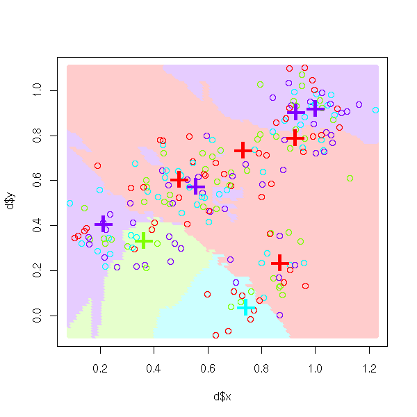
TODO: plot the theoretical boundary.
TODO: there is already a package for this...
library(help=knnTree)
Exercice: use a kernel instead.
TODO: Read chapter 4 of "The Elements of Statistical Learning"
TODO
library(mda)
?mda
TODO
library(mda)
?fda
We consider two binary random variables X and Y and we try to predict Y from X.
For instance, we try to predict the name of a fruit from its shape.
X = "round" or "long"
Y = "apple" or "non-apple" (e.g.: bananam, orange)
We have a set of fruits to learn to recognise them: we know their shape and we know if they are an apple or not. For instance:
     |  pomme  |  pas une pomme
-----+---------+-----------------
rond |         |
-----+---------+-----------------
long |         |

TODO: choose numeric values
When we see a new fruit, we can try to guess wether it is an apple in the following way: we compute the conditionnal probabilities
                             P( Y = apple et X = round )
P( Y = apple | X = round ) = ----------------------------
                                   P( X = round )

                                 P( Y = non-apple et X = round )
P( Y = non-apple | X = round ) = --------------------------------
                                         P( X = round )
and we conpare them. If the first is the larger, we shall say it is an apple, if it is the second, we shall say it is not.
With our values:
TODO
All the presentations of the naive Bayes classifier relie on the Bayes formula. Indeed, the formula we have use,
                             P( Y = apple et X = round )
P( Y = apple | X = round ) = ----------------------------
                                   P( X = round )
can also be written
                             P( X = round | Y = apple ) * P( Y = Apple )
P( Y = apple | X = round ) = --------------------------------------------
                                           P( X = round )
which is called "the Bayes formula".
When we only had one predictive variable, it was not that useful, but we shall see that with several, it becomes handy.
This idea can easily be generalized to several predictive variables (shape of the fruit, colour, pips or stone, etc.).
                           P(X1=b1 and ... and Xn=bn and Y=a)
P(Y=a|X=(b1,b2,...,bn)) = ---------------------------------
                               P(X1=b1 and ... and Xn=bn)
But, if there are many predictive variables, some problems may occur: in some cases, we have not observed simultaneously b1, b2, ..., and bn. What can we do?
It is here that conditionnal probabilities really become useful.
                           P(X=(b1,...,bn)|Y=a) * P(Y=a)
P(Y=a|X=(b1,b2,...,bn)) = -------------------------------
                                  P(X=(b1,...,bn))
If the Xi are independant (it is a reasonnable hypothesis, iven if it is false: otherwise, we would have to investigate the dependancy relations, the interactions, between the Xi -- this would require much more data), this can be written
                           P(X1=b1|Y=a) * ... * P(Xn=bn|Y=a) * P(Y=a)
                        = --------------------------------------------
                                         P(X=(b1,...,bn))
We are interested in the value of a tha maximizes this quantity. As a does not appear in the denominator, we can get rid of it and find the value of a that maximizes the numerator
P(X1=b1|Y=a) * ... * P(Xn=bn|Y=a) * P(Y=a).
A naive bayesian classifier will thus be used in two steps: first, compute the conditionnal probabilities
P(Xi=bj|Y=a)
for all the values of i, j and a and the a priori probabilities
P(Y=a)
from the learning data set and then, in a second step, given new values for the Xi, find the value of a that maximizes
P(X1=b1|Y=a) * ... * P(Xn=bn|Y=a) * P(Y=a).
We had to assume that the predictive variables were independant (this is the meaning of the word "naive" in the expression "naive Bayes classifier"). This hypothesis is usually wrong -- however, the forecasts are nonetheless rather reliable.
http://www.cs.washington.edu/homes/pedrod/mlj97.ps.gz

TODO: read this document...
As the idea is relatively simple, we can easily implement ourselves such a predictor.
my.bayes <- function (y, x, xp) {
  # TODO:
  # we should check that y, the columns of x and xp are factors,
  # that xp and x have the same number of columns,
  # that the levels of the columns of xp and x are the same
  # (or at least that the values in the columns of xp are among the
  # levels of x)
  na <- names(x)
  m <- dim(x)[2]
  # Compute the conditionnal probabilities
  pc <- list()
  for (i in 1:m) {
    a <- table(data.frame(y,x=x[,i]))
    a <- a / apply(a,1,sum)
    pc[[ na[i] ]] <- a
  }
  # Compute the a priori probabilities
  pap <- table(y)
  pap <- pap/sum(pap)
  # To avoid numerical instability, we consider sums of logarithms
  # of probabilities instead of products of probabilities
  pc <- lapply(pc,log)
  pap <- log(pap)
  # Compute the P(X1=b1|Y=a) * ... * P(Xn=bn|Y=a) * P(Y=a)
  papo <- matrix(0, nr=dim(xp)[1], nc=length(pap))
  colnames(papo) <- names(pap)
  # I am sure we could do this with no loop...
  for (i in 1:dim(xp)[1]) {
    for (j in 1:length(pap)) {
      papo[i,j] <- pap[j]
      for (k in 1:dim(x)[2]) {
        papo[i,j] <- papo[i,j] + pc[[ na[k] ]][j,xp[i,k]]
      }
    }
  }
  papo <- papo - apply(papo,1,mean)
  papo <- exp(papo)
  levels(y)[ apply(papo, 1, function (a) { which(a==max(a))[1] }) ]
}

# Data
library(e1071)
data(HouseVotes84)
y <- HouseVotes84[,1]
x <- HouseVotes84[,-1]
# Err...
# I forgot to account for missing value
i <- which(!apply( apply(x,1,is.na), 2, any ))
x <- x[i,]
y <- y[i]

# Compute the forecasts: correct in 92% of the cases.
yp <- my.bayes(y,x,x)
mean(y==yp)
Actually, it is already there -- and the function, contrary to ours, accounts for missing values.
library(e1071)
?naiveBayes
For sample data, have a look at
library(mlbench)
data(package=mlbench)
TODO: recall what it is
library(mlbench)
data(DNA)
d <- DNA
d$Class <- factor(ifelse(d$Class=='n','n','i'))
library(e1071)
r <- naiveBayes(Class~.,d)
i <- sample(1:dim(d)[2],100)
p <- predict(r, d[,-length(d)][i,])       # Long...
A <- sum(p == 'i' & d$Class[i] == 'i')
B <- sum(p == 'i' & d$Class[i] != 'i')
C <- sum(p != 'i' & d$Class[i] == 'i')
# Precision rate
100 * A/(A+B)
# Recall rate
100 * A/(A+C)
TODO

library(mlbench)
data(DNA)
d <- DNA
d$Class <- factor(ifelse(d$Class=='n','n','i'))
library(e1071)
r <- naiveBayes(Class~.,d)
p <- predict(r, d[,-length(d)], type='raw')
For several years, bayesian classifiers have been used in mail filters -- the interesting point is that they learn the kind of mail _you_ receive and the kind of spam that flood the web -- everyone ends up with a different filter.
http://www.paulgraham.com/spam.html
http://www.xml.com/pub/a/2003/11/19/udell.html

K. Williams, An Introduction to Machine Learning with Perl
http://conferences.oreillynet.com/presentations/bio2003/williams_ken.ppt
The variable to predict, Y, has two values: "spam" and "non-spam". There is a predictive variable for each word (yes, that means thousands of predictive variables -- actually, we shall restrict ourselves to the most common words and end up with hardly more than one thousand words), with two values: "present" or "absent".
The learning step is carried out from messages whose nature is known -- for instance, the messages you received last week).
More generally, text classification is one of the main applications of the naive Bayes classifier
TODO: give other examples (URL)
There is another notion of a "naive Bayes classifier", in which the predictive variables are quantitative: these are counting variables -- in the spam example or in the text classification example, we not only look at the presence/absence of a word, but also hoz many times it occurs.
Should you wish to distinguish the two classifiers, you can can the binary one "Binomial Naive Bayes Classifier" and the counting variable one "Multinomial Naive Bayes Classifier".
A. McCallum, K. Nigam
A Comparison of Event Models for Naive Bayes Text Classification
http://www-2.cs.cmu.edu/%7Eknigam/papers/multinomial-aaaiws98.pdf
There are variants of the naive Bayes classifier that tackle its overly naive hypothesis (the independance of the predictive variables).
TAN (Tree-augmented Naive Bayes) model the dependance relations between predictive variables by a tree.
Bayesian networks (very trendy for a couple of years, as were the neural networks in tge 1990s) model the dependance relations between the predictive variables by a graph.
http://www.vision.ethz.ch/gm/bnclassifiers.pdf

The Holmes and Watson examples (they are actually taken from Finn
Jensen's book: An introduction to Bayesian Networks):
http://www.ai.mit.edu/courses/6.825/fall02/pdf/6.825-lecture-15.pdf
More generally, Bayesian classifiers may be used with any classification problem.
1. We want to know if a family name comes from southern Asia or not. For this, we look at the presence/absence of 4-letter strings in the name.
http://dimax.rutgers.edu/%7Esguharay/newfinalpresentation.pdf
2. Handwritten character recognition, on a PDA.
3. Voice recognition, on a mobile phone.
4. We have a bunch of biology research article abstracts and we are looking for sentences that describe gene interactions. To this end, we process by hand a few hundred sentences: we look at the words it contains (our predictive variables) and we state if it describes a gene interaction (our variable to predict). From this learning corpus, we compute the conditionnal and a priori probabilities. Given a new sentence, the Bayes classifier gives us the probability that it describes an interaction.
http://zoonek2.free.fr/bioinfo/TM/rapport.pdf
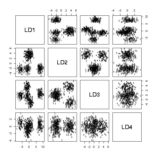
We have already mentionned it above: we want to predict a qualitative variable from several quantitative variables. More geometrically, we are looking for a plane (or a subspace of smaller dimension) in which the various values of the quantitaive variable correspond to points as far away as possible.
library(MASS)
n <- 100
k <- 5
x1 <- runif(k,-5,5) + rnorm(k*n)
x2 <- runif(k,-5,5) + rnorm(k*n)
x3 <- runif(k,-5,5) + rnorm(k*n)
x4 <- runif(k,-5,5) + rnorm(k*n)
x5 <- runif(k,-5,5) + rnorm(k*n)
y <- factor(rep(1:5,n))
plot(lda(y~x1+x2+x3+x4+x5))
Regression with quantitative variables can be written
E(Y) = a0 + a1 x1 + ... + an xn.
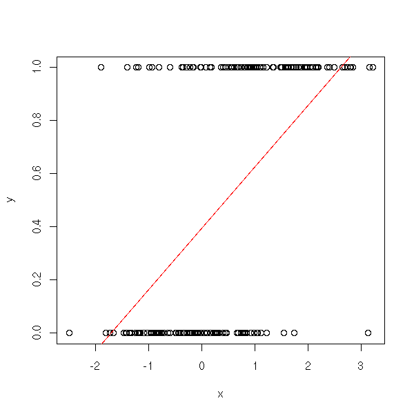
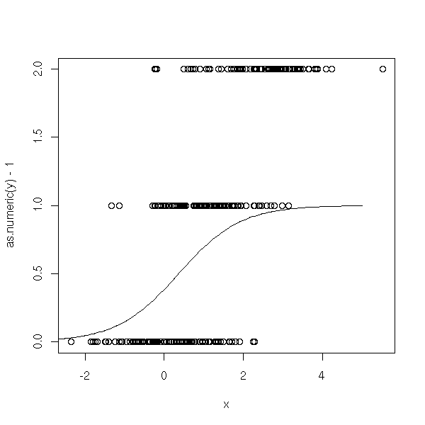
But if Y only has a finite number of variables, this is no longer relevant: we can use numbers for the values of Y, but Y will be bounded, will only assume a fixed number of values, known in advance, while the right hand side of the expression is not bounded and can take an infinite number of values -- it does not look very serious and can become troublesome when you want to predict Y.
n <- 100
x <- c(rnorm(n), 1+rnorm(n))
y <- c(rep(0,n), rep(1,n))
plot(y~x)
abline(lm(y~x), col='red')
The idea of the Generalized Model (GLM)) is to replace E(Y) by something else.
For logistic regression, the variable to predict, Y, has only two values, 0 and 1, and we are interested in the probability of each.
P[ Y == 1 ] = a0 + a1 x1 + ... + an xn.
Hardly better: actually, it is the same formula (because E(Y)=P(Y==1)) and we have the same problem: the left hand side is bounded, the right hand side is not. To get rid of the problem, we can apply some transformation to the left hand side, a bijection between the interval (0,1) and the real line -- in GLM parlance, such a function is called a "link".
One often uses the logistic function>
                  p
logit(p) = log -------
                1 - p
We can write
                        P(win)
logit( P(winr) ) = log --------.
                        P(lose)
The quotient P(win)/P(lose) is called the "odds" (bookmakers often use this expression: "the odds are 3 to 1", etc.)
Here is the plot of this function.
x <- seq(0,1, length=100)
x <- x[2:(length(x)-1)]
logit <- function (t) {
  log( t / (1-t) )
}
plot(logit(x) ~ x, type='l')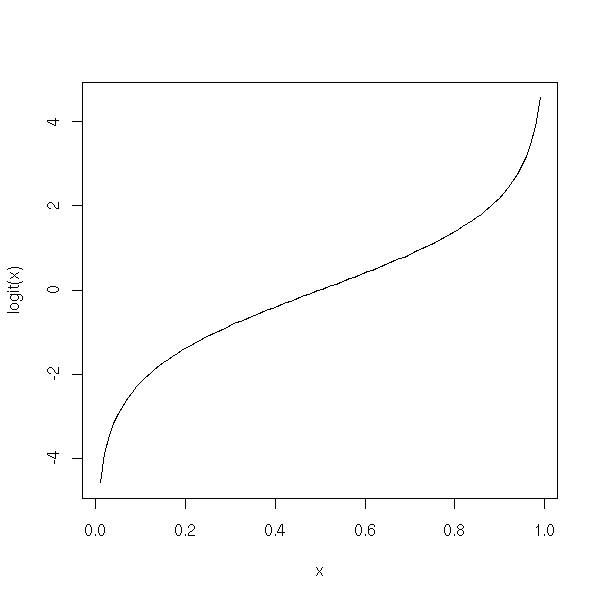
The "probit" function, the inverse of the cumulative distribution function of the gaussian distribution, is another link.
curve(logit(x), col='blue', add=F)
curve(qnorm(x), col='red', add=T)
a <- par("usr")
legend( a[1], a[4], c("logit","probit"), col=c("blue","red"), lty=1)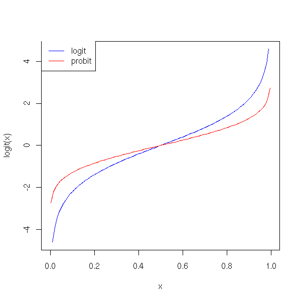
The "log-log" function is yet another link.
curve(logit(x), col='blue', add=F)
curve(qnorm(x), col='red', add=T)
curve(log(-log(1-x)), col='green', add=T)
abline(h=0, lty=3)
abline(v=0, lty=3)
a <- par("usr")
legend( a[1], a[4],
        c("logit","probit", "log-log"),
        col=c("blue","red","green"),
        lty=1)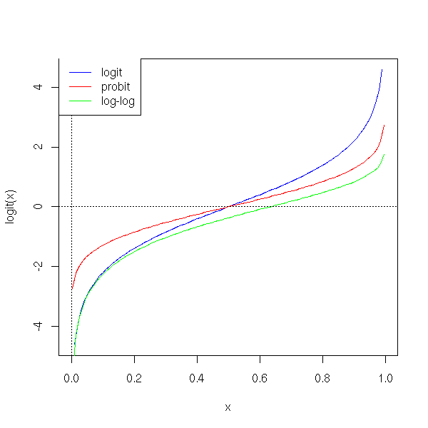
You might also think about transforming the data with the inverse of the link function, perform a linear regression and apply the link to the result. It would not work, because the initial data are 0 and 1 and would give infinite values -- we are no longer trying to model the data values themselves, but their probabilities.
ilogit <- function (l) {
  exp(l) / ( 1 + exp(l) )
}
fakelogit <- function (l) {
  ifelse(l>.5, 1e6, -1e6)
}
n <- 100
x <- c(rnorm(n), 1+rnorm(n))
y <- c(rep(0,n), rep(1,n))
yy <- fakelogit(y)
xp <- seq(min(x),max(x),length=200)
yp <- ilogit(predict(lm(yy~x), data.frame(x=xp)))
yp[is.na(yp)] <- 1
plot(y~x)
lines(xp,yp, col='red', lwd=3)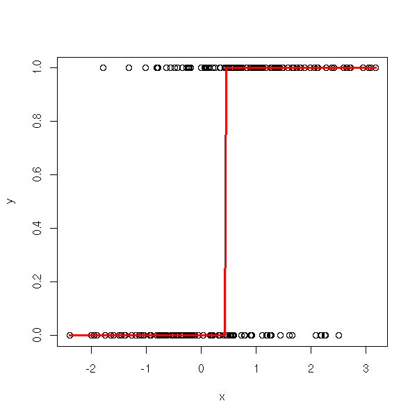
So we give up Least Squares Estimation and compute a Maximum Likelihood Estimator.
n <- 100
x <- c(rnorm(n), 1+rnorm(n))
y <- c(rep(0,n), rep(1,n))
f <- function (a) {
  -sum(log(ilogit(a[1]+a[2]*x[y==1]))) - sum(log(1-ilogit(a[1]+a[2]*x[y==0])))
}
r <- optim(c(0,1),f)
a <- r$par[1]
b <- r$par[2]
plot(y~x)
curve( dnorm(x,1,1)*.5/(dnorm(x,1,1)*.5+dnorm(x,0,1)*(1-.5)), add=T, col='red')
curve( ilogit(a+b*x), add=T )
legend( .95*par('usr')[1]+.05*par('usr')[2],
        .9,
        c('theoretical curve', 'MLE'),
        col=c('red', par('fg')),
        lty=1, lwd=1)
title(main="Logistic regression, by hand")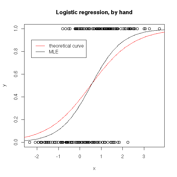
This can be done directly, with the "glm" function.
#
# BEWARE:
# Do not forget the "family" argument -- otherwise, it would be a
# linear regression -- the very thing we are trying to avoid.
#
r <- glm(y~x, family=binomial)
plot(y~x)
abline(lm(y~x),col='red',lty=2)
xx <- seq(min(x), max(x), length=100)
yy <- predict(r, data.frame(x=xx), type='response')
lines(xx,yy, col='blue', lwd=5, lty=2)
lines(xx, ilogit(r$coef[1]+xx*r$coef[2]))
legend( .95*par('usr')[1]+.05*par('usr')[2],
        .9,
        c('linear regression',
          'prediction with "predict"',
          "prediction with the coefficients"),
        col=c('red', 'blue', par('fg')),
        lty=c(2,2,1), lwd=c(1,5,1))
title(main='Logistic regression with the "glm" function')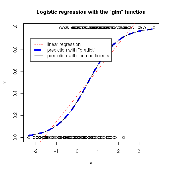
In particular, the predicted values, which are probabilities, are indeed between 0 and 1 -- with linear regression, they were not bounded.
We can compare the various kinds of regression: logistic regression yields the results closer to the theoretical curve.
n <- 100
x <- c(rnorm(n), 1+rnorm(n))
y <- c(rep(0,n), rep(1,n))
plot(y~x)
# Brutal prediction
m1 <- mean(x[y==0])
m2 <- mean(x[y==1])
m <- mean(c(m1,m2))
if(m1<m2) a <- 0
if(m1>m2) a <- 1
if(m1==m2) a <- .5
lines( c(min(x),m,m,max(x)),
       c(a,a,1-a,1-a),
       col='blue')
# Linear regression
abline(lm(y~x), col='red')
# Logistic regression
xp <- seq(min(x),max(x),length=200)
r <- glm(y~x, family=binomial)
yp <- predict(r, data.frame(x=xp), type='response')
lines(xp,yp, col='orange')
# Theoretical curve
curve( dnorm(x,1,1)*.5/(dnorm(x,1,1)*.5+dnorm(x,0,1)*(1-.5)), add=T, lty=3, lwd=3)
legend( .95*par('usr')[1]+.05*par('usr')[2],
        .9, #par('usr')[4],
        c('Brutal prediction', "Linear regression", "Logistic regression",
          "Theoretical curve"),
        col=c('blue','red','orange', par('fg')),
        lty=c(1,1,1,3),lwd=c(1,1,1,3))
title(main="Comparing linear and logistic regression")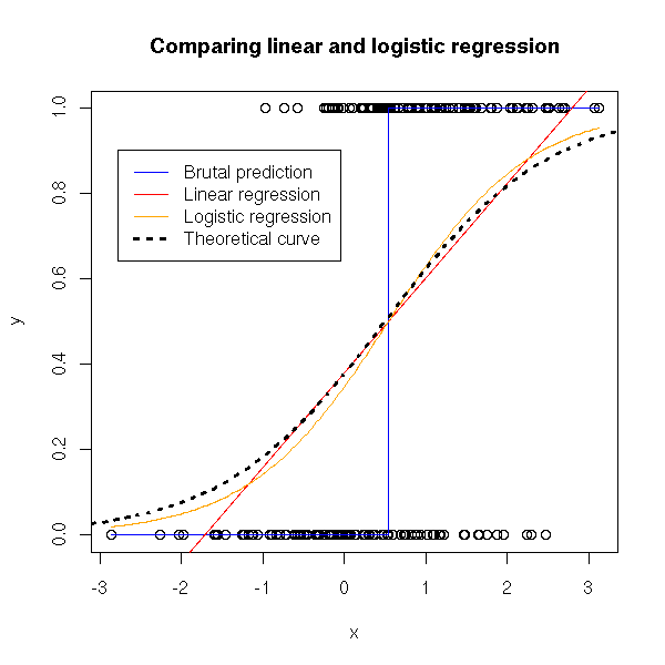
Do not forget to have a look at the examples from the "glm" manual:
demo("lm.glm")TODO: Compare the various links.
As for linear regression, we have three means of displaying the result.
The "print" function":
> r

Call:  glm(formula = y ~ x, family = binomial)

Coefficients:
(Intercept)            x
    -0.4864       0.9039

Degrees of Freedom: 199 Total (i.e. Null);  198 Residual
Null Deviance:      277.3
Residual Deviance: 239.7        AIC: 243.7
The "summary" function:
> summary(r)

Call:
glm(formula = y ~ x, family = binomial)

Deviance Residuals:
     Min        1Q    Median        3Q       Max
-1.94200  -0.99371   0.05564   0.97949   1.87198

Coefficients:
            Estimate Std. Error z value Pr(>|z|)
(Intercept)  -0.4864     0.1804  -2.696  0.00702 **
x             0.9039     0.1656   5.459 4.79e-08 ***
---
Signif. codes:  0 `***' 0.001 `**' 0.01 `*' 0.05 `.' 0.1 ` ' 1

(Dispersion parameter for binomial family taken to be 1)

    Null deviance: 277.26  on 199  degrees of freedom
Residual deviance: 239.69  on 198  degrees of freedom
AIC: 243.69

Number of Fisher Scoring iterations: 3
The "anova" function:
> anova(r)
Analysis of Deviance Table

Model: binomial, link: logit

Response: y

Terms added sequentially (first to last)

      Df Deviance Resid. Df Resid. Dev
NULL                    199    277.259
x      1   37.566       198    239.693
There is also the "aov" function.
> aov(r)
Call:
   aov(formula = r)

Terms:
                       x Residuals
Sum of Squares   9.13147  40.86853
Deg. of Freedom        1       198

Residual standard error: 0.45432
Estimated effects may be unbalanced
Let us also mention the "manova" function.
?summary.manova
As usual, we have a wealth of plots to assess the quality of the regression results.
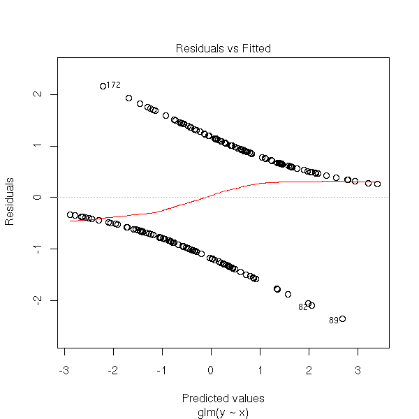
The Pearson residuals are defined as
         y_i - \hat y_i
r_i =   ----------------
              s_i
where s_i is the estimation of the standard deviation of the noise. There is also a normalized version (this is the same sa with linear regression: the standard deviation of the noise and the standard deviation of the residuals are different) and a standardized version (we divide by the estimation of the standard deviation obtained by removing observation "i").
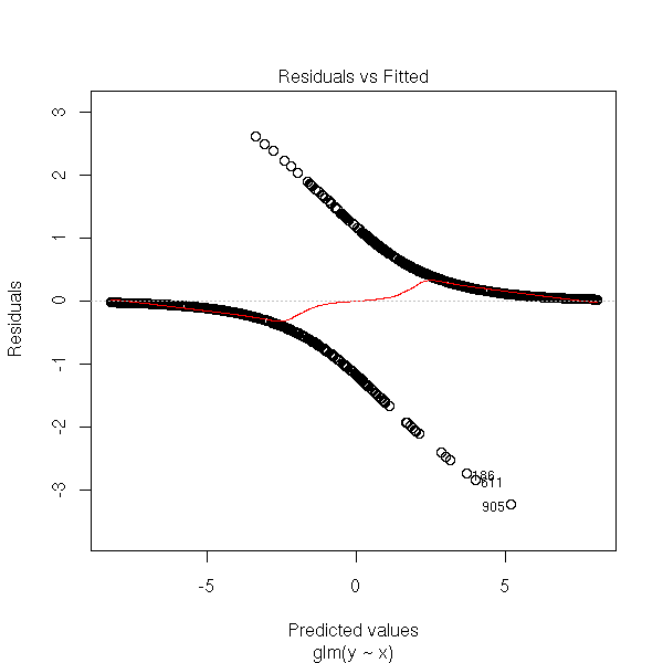
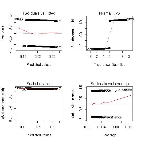
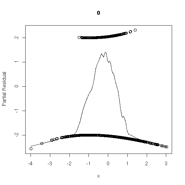
You will notice that y_i is 0 or 1, while \hat y_i is a probability (between 0 and 1), which explains the shape of the plot: se see two curves, one above the axis, the other under, that correspond to the two possible values of y_i. One of those curves is decreasing and tends to 0 in + infinity, for the other, it is the opposite.
n <- 100
x <- c(rnorm(n), 1+rnorm(n))
y <- c(rep(0,n), rep(1,n))
r <- glm(y~x, family=binomial)
plot(r, which=1)
Actually, this simulation does not faithfully reflect the model underlying the logistic regression. It would rather be like this:
n <- 1000
a <- -2
b <- 1
x <- runif(n, -4, 5)
y <- exp(a*x+b + rnorm(n))
y <- y/(1+y)
y <- rbinom(n,1,y)
plot(y~x)
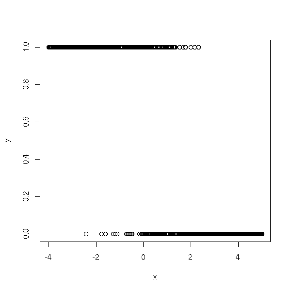
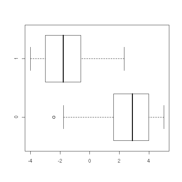
boxplot(x~y, horizontal=T)
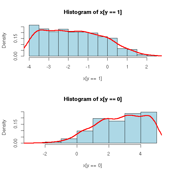
op <- par(mfrow=c(2,1))
hist(x[y==1], probability=T, col='light blue')
lines(density(x[y==1]),col='red',lwd=3)
hist(x[y==0], probability=T, col='light blue')
lines(density(x[y==0]),col='red',lwd=3)
par(op)
rt <- glm(y~x, family=binomial)
plot(rt, which=1)
TODO: give concrete examples of pathological situations.
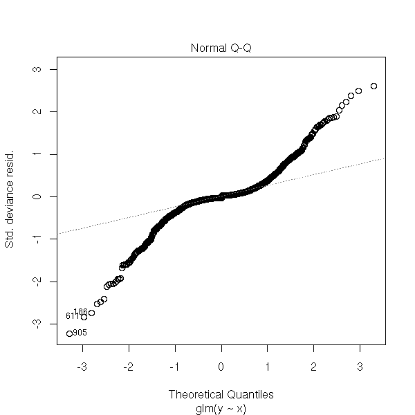
We are also suggested to look at the gaussian quantile-quantile plot of the residuals -- but I do not understand whym because the residuals are not supposed to be gaussian.
plot(rt, which=2)
hist(rt$residuals, breaks=seq(min(rt$residuals),max(rt$residuals)+1,by=.5),
     xlim=c(-10,10),
     probability=T, col='light blue')
points(density(rt$residuals, bw=.5), type='l', lwd=3, col='red')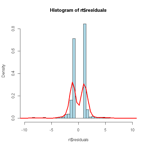
However, one can transform those residuals to get a gaussian distribution: these are the Anscombe residuals -- the transformation is rather complex and R does not seem to know it...
Exercice: implement this transformation, in an approximate manner, with a simulation.
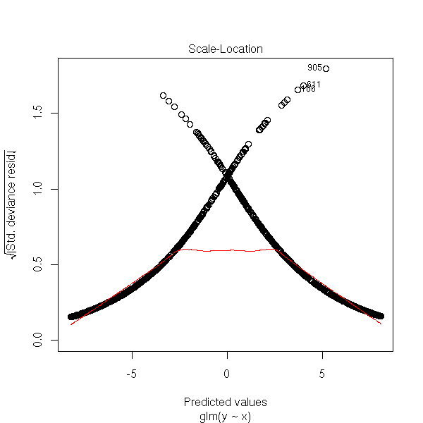
We can also look at the absolute value of the residuals.
plot(rt, which=3)
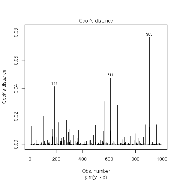
and the Cook distances.
plot(rt, which=4)

The deviance is defined by
D = -2(L-Lsat)
where L is the log-likelihood of our model and Lsat the log-likelihood of the saturated model (with as many variables as observations).
TODO: understand. (Where do those new variables come from?)
We are happy if D/df < 1.
> rt$deviance
[1] 362.0677
We also have the deviance of the null model (the model with no variables, corresponding to the hypothesis "the predictive variables have no effect"), i.e., the probability of Y=1 is constant and does not depend on the predictive variables).
> rt$null.deviance
[1] 1383.377
The AIC (Akaike Information Criterion) is preferable to the deviance to compare models, because it accounts for the number of parameters in those models.
> rt$aic
[1] 366.0677
It is defined by
- 2 * log-likelihood + 2 * number of parameters.
There are a few variants, such as the BIC,
- 2 * log-likelihood + ln(number of observations) * number of parameters.
We have already seen the various residuals.
Pearson residuals (aka raw residuals, standardized residuals, studentized residuals):
 y_i - \hat y_i
----------------
      s_i
Deviance residuals: contribution of each observation to the deviance.
Anscombe residuals: we transform the variable to that the residuals follow a gaussian distribution (the "t" function is complicated):
t(y_i) - t(\hat y_i)
----------------------
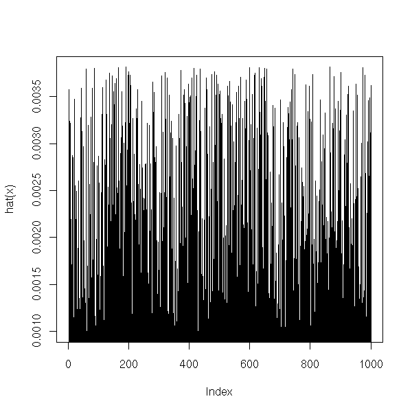
t'(y_i) s_iAs with linear regression, we can measure the leverage, with the "hat matrix" (but it is not exactly the same matrix).
TODO: with R

# It is supposed not to be the same as in the linear situation.
# Here, it seems to be the same...
plot(hat(x), type='h')
We also have the Cook distance, as for linear regression.
plot(rt, which=4)
Likelihood Ratio test: to compare two nested models with q1 and q2 parameters,we look at D2 - D2, that asymptotically follows a Chi^2 distribution (if we start with a binomial or Poisson distribution) or a Fisher distribution (if we start with a gaussian distribution) with q2 - q1 degrees of freedom.
TODO: understand
Wald test: it is a quadratic approximation of the Likelihood Ratio test.
library(car)
?linear.hypothesis
(Answer to a question I was asked by email)
Let us consider the data
library(mlbench)
data(BostonHousing)
y <- BostonHousing[,1]
y <- factor(y>median(y))
x1 <- BostonHousing[,2]
x2 <- BostonHousing[,3]
We can compute the logistic regression with the "glm" function.
glm(y~x1+x2, family=binomial)
or with the "lrm" function in the "Design" package, that provides much more information.
library(Design)
lrm(y~x1+x2)
This yields:
> lrm(y~x1+x2)
Logistic Regression Model

lrm(formula = y ~ x1 + x2)

Frequencies of Responses
FALSE  TRUE
  253   253

     Obs  Max Deriv Model L.R.       d.f.          P          C        Dxy
     506      3e-06     234.13          2          0      0.862      0.724
   Gamma      Tau-a         R2      Brier
   0.725      0.363      0.494      0.145

          Coef     S.E.    Wald Z P
Intercept -1.66990 0.27245 -6.13  0e+00
x1        -0.04954 0.01280 -3.87  1e-04
x2         0.17985 0.02084  8.63  0e+00
Question:
> 1. In a logistic regression, how do we know if the model is
> "good"? I.e., do we have an equivalent of the R^2?
There are several equivalents of the R^2 for logistic regression. The simplest, "pseudo-R^2" or "McFadden's R^2" is
 (deviance of the model) - (deviance of the null model)
--------------------------------------------------------
              (deviance of the null model)
I recall that the deviance is
- 2 log(L)
where L is the likelihood and that the "null model" is "y ~1" (the model with no predictive variables, the model that assumes that the quantities we are modelling (the probability of Y) are constant).
It can be interpreted as the "proportion of the deviance explained by the model" -- similarly, the R^2 was the "proportion of variance explained by the model".
But it does not tell you if the model is good: if the R^2 is low, it can mean that there is a lot of noise or that the model is incomplete.
The idea is the same as for linear models: plots. To learn how to read them, let us start with a few simulations.
Random data:
n <- 1000
y <- factor(sample(0:1,n,replace=T))
x <- rnorm(n)
r <- glm(y~x,family=binomial)
op <- par(mfrow=c(2,2))
plot(r,ask=F)
par(op)
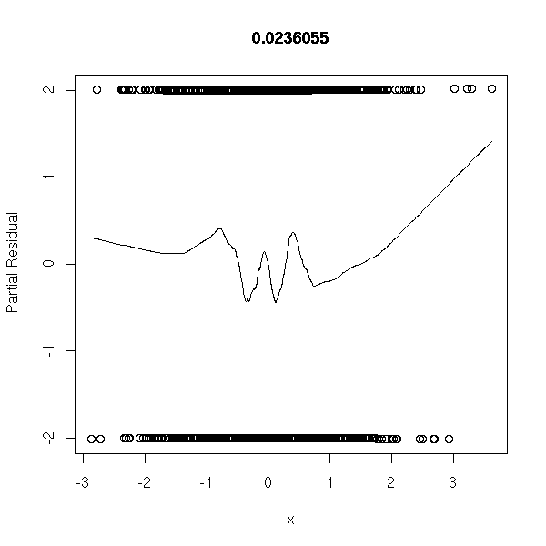
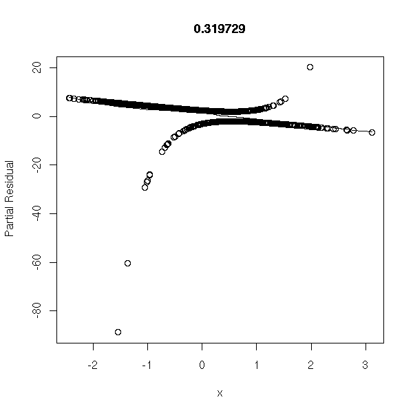
library(Design)
r <- lrm(y~x,y=T,x=T)
P <- resid(r,"gof")['P']
resid(r,"partial",pl=T)
title(signif(P))
Data coming from the model:
n <- 1000
x <- rnorm(n)
a <- 1
b <- -2
p <- exp(a+b*x)/(1+exp(a+b*x))
y <- factor(ifelse( runif(n)<p, 1, 0 ), levels=0:1)
r <- glm(y~x,family=binomial)
op <- par(mfrow=c(2,2))
plot(r,ask=F)
par(op)
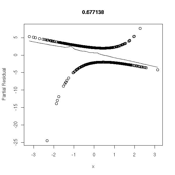
r <- lrm(y~x,y=T,x=T)
P <- resid(r,"gof")['P']
resid(r,"partial",pl=T)
title(signif(P))
Data from the model, with random errors (I do not see anything on the plot, but the estimators of a and b are biased towards zero):
n <- 1000
x <- rnorm(n)
a <- 1
b <- -2
p <- exp(a+b*x)/(1+exp(a+b*x))
y <- ifelse( runif(n)<p, 1, 0 )
i <- runif(n)<.1
y <- ifelse(i, 1-y, y)
y <- factor(y, levels=0:1)
col=c(par('fg'),'red')[1+as.numeric(i)]
r <- glm(y~x,family=binomial)
op <- par(mfrow=c(2,2))
plot(r,ask=F, col=col)
par(op)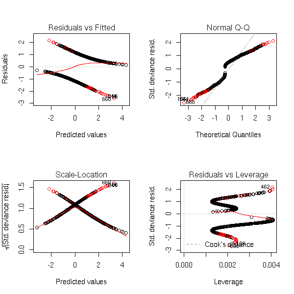
r <- lrm(y~x,y=T,x=T)
P <- resid(r,"gof")['P']
resid(r,"partial",pl=T)
title(signif(P))
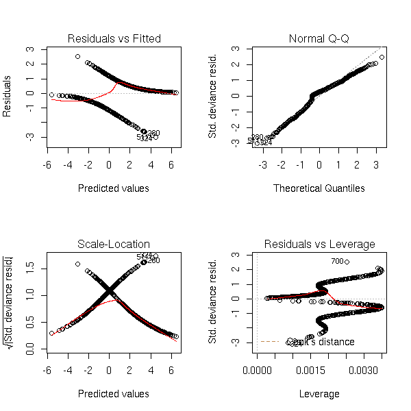
Data from the model, with mode extreme errors:
n <- 1000
x <- rnorm(n)
a <- 1
b <- -2
p <- exp(a+b*x)/(1+exp(a+b*x))
y <- ifelse( runif(n)<p, 1, 0 )
i <- runif(n)<.5 & abs(x)>1
y <- ifelse(i, 1-y, y)
y <- factor(y, levels=0:1)
col=c(par('fg'),'red')[1+as.numeric(i)]
r <- glm(y~x,family=binomial)
op <- par(mfrow=c(2,2))
plot(r,ask=F, col=col)
par(op)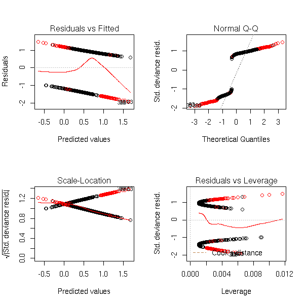
r <- lrm(y~x,y=T,x=T)
P <- resid(r,"gof")['P']
resid(r,"partial",pl=T)
title(signif(P))
One variable too many:
n <- 1000
x1 <- rnorm(n)
x2 <- rnorm(n)
a <- 1
b <- -2
p <- exp(a+b*x1)/(1+exp(a+b*x1))
y <- factor(ifelse( runif(n)<p, 1, 0 ), levels=0:1)
r <- glm(y~x1+x2,family=binomial)
op <- par(mfrow=c(2,2))
plot(r,ask=F)
par(op)
r <- lrm(y~x,y=T,x=T)
P <- resid(r,"gof")['P']
resid(r,"partial",pl=T)
title(signif(P))
Non-linear model:
n <- 1000
x <- rnorm(n)
a <- 1
b1 <- -1
b2 <- -2
p <- 1/(1+exp(-(a+b1*x+b2*x^2)))
y <- factor(ifelse( runif(n)<p, 1, 0 ), levels=0:1)
r <- glm(y~x,family=binomial)
op <- par(mfrow=c(2,2))
plot(r,ask=F)
par(op)
r <- lrm(y~x,y=T,x=T)
P <- resid(r,"gof")['P']
resid(r,"partial",pl=T)
title(signif(P))
Well, those plots seem much less useful than they were for linear regression.
Question:
> 2. What about the Wald, Hosmer and Lemshow, Somer's D tests?
> What do they test? How do we compute them? How do we interpret
> them?
The Wald test I know (there might be another one with the same name) is an approximation of the likelihood ratio test: prefer the genuine one.
The likelihood ratio test compares two nested models whose parameters have been estimated by the maximum likelihood method. In R, it is computed by the "anova" function. (The "F test" comparing a linear model to the trivial model is a particular case of it.)
We would expect to be able to perform this test as with linear models:
r <- glm(y~x1+x2, family=binomial())
anova(r)
but no...
You can perform the test by hand: the difference of the deviances of two nested models (here, the model we are interested in and the null model) follows, asymptotically, a Chi^2 distribution with p degrees of freedom, where p is the number of parameters that are fixed in the smaller model.
r <- glm(y~x1+x2, family=binomial())
pchisq(r$null.deviance - r$deviance, df=2, lower.tail=F)
You can use this test to compare two non-trivial models -- but they have to be nested.
r0 <- glm(y~x1+x2, family=binomial)
r1 <- glm(y~x1, family=binomial)
r2 <- glm(y~x2, family=binomial)
lr.test <- function (r.petit,r.gros) {
  pchisq(r.petit$deviance - r.gros$deviance, df=1, lower.tail=F)
}
lr.test(r1,r0)
lr.test(r2,r0)
Here, we find that the model y ~ x1+x2 is significantly better that y ~ x1, with a risk of error inferior to 1e-21, and that the model y~x1+x2 is significantly better than y~x2, with a risk of error under 1e-6.
Actually, the "lrm" function (in the Design package) already performs this test.
lrm(y~x1+x2)
In our example,
     Obs  Max Deriv Model L.R.       d.f.          P          C        Dxy
     506      3e-06     234.13          2          0      0.862      0.724
   Gamma      Tau-a         R2      Brier
   0.725      0.363      0.494      0.145
the p-value is zero, so the model is significantly better than the trivial one.
I think that "Wald's test" also refers to the test checking if a regression coefficient is zero (under the null hypothesis that this coefficient is zero, the estimated coefficient, divided by its standard deviation, follows a gaussian distribution; if you square it , it follows a Chi^2 distribution with one degree of freedom). Thus, if we look at the last column of the result of the previous function,
          Coef     S.E.    Wald Z P
Intercept -1.66990 0.27245 -6.13  0e+00
x1        -0.04954 0.01280 -3.87  1e-04
x2         0.17985 0.02084  8.63  0e+00
you can tell that the intercept and the x2 coefficient are non-zero with a negligible risk of error and that the x1 coefficient is non-zero with a risk of error of 0.1%.
Actually, we already had those results with the "glm" function:
> summary(r0)
Call:
glm(formula = y ~ x1 + x2, family = binomial)

Deviance Residuals:
    Min       1Q   Median       3Q      Max
-2.5902  -0.7571   0.1312   0.6106   2.0397

Coefficients:
            Estimate Std. Error z value Pr(>|z|)
(Intercept) -1.66990    0.27245  -6.129 8.84e-10 ***
x1          -0.04954    0.01280  -3.870 0.000109 ***
x2           0.17985    0.02084   8.632  < 2e-16 ***

(Dispersion parameter for binomial family taken to be 1)

    Null deviance: 701.46  on 505  degrees of freedom
Residual deviance: 467.33  on 503  degrees of freedom
AIC: 473.33

Number of Fisher Scoring iterations: 6
I have never heard of the Hosmer and Lemeshow test, but Google refers me to
http://www.biostat.wustl.edu/archives/html/s-news/1999-04/msg00147.html
http://maths.newcastle.edu.au/~rking/R/help/03b/0735.html
http://www.learnlink.mcmaster.ca/OpenForums/00031830-80000001/00040559-80000001/0045CA16-00977198-005B1B21
which claim that this test is obsolete. The "residuals.lrm" function in the Design package has a test to replace it -- but I do not know what is behind it, neither how to interpret it.
library(Design)
?residuals.lrm
For our example:
> resid( lrm(y~x1+x2, y=T, x=T), "gof" )
Sum of squared errors     Expected value|H0                    SD
         7.328945e+01          7.632820e+01          5.739924e-01
                    Z                     P
        -5.294060e+00          1.196300e-07
I do not know Somers's D, but some simulations can help interpret it.
> library(Design)
> somers2(x1,as.numeric(y)-1)
          C         Dxy           n     Missing
  0.2846475  -0.4307051 506.0000000   0.0000000
> somers2(-x1,as.numeric(y)-1)
          C         Dxy           n     Missing
  0.7153525   0.4307051 506.0000000   0.0000000
> somers2(x2,as.numeric(y)-1)
          C         Dxy           n     Missing
  0.8551532   0.7103064 506.0000000   0.0000000
> somers2(-x2,as.numeric(y)-1)
          C         Dxy           n     Missing
  0.1448468  -0.7103064 506.0000000   0.0000000
> somers2(rnorm(506),as.numeric(y)-1)
           C          Dxy            n      Missing
  0.50564764   0.01129529 506.00000000   0.00000000
It seems to be interpretable as a correlation, when one of the variables only has two values, 0 and 1.
So we have the same problems as with correlation: it is only relevant for linear relations. Thus the following computations give (approximately) 1 and 0.
n <- 1000
a <- rnorm(n)
b <- ifelse(a<0,0,1)
somers2(a,b)

b <- ifelse(abs(a)<.5,0,1)
somers2(a,b)
# age
age <- c(25.0, 32.5, 37.5, 42.5, 47.5, 52.5, 57.5, 65.0)
# Number of successes
n <- c(100, 150, 120, 150, 130, 80, 170, 100)
# predictive variable
Y <- c(10, 20, 30, 50, 60, 50, 130, 80)

f<-Y/n
g<-log(f/(1-f)) # Transforming the data
w<-n*f*(1-f) # Weights
r<-predict(lm(g~age,weights=w)) # Weighted regression
p<-exp(r)/(1+exp(r)) # Inverse transform
plot(age,f,ylim=c(0,1))
lines(age,p)
symbols(age,f,circles=w,add=T)
# Iterate...
w<-n*p*(1-p)
gu<-r+(f-p)/p/(1-p)
r<-predict(lm(gu~age,weights=w))
# Once more
p<-exp(r)/(1+exp(r))
w<-n*p*(1-p)
gu<-r+(f-p)/p/(1-p)
r<-predict(lm(gu~age,weights=w))
Actually, we get the results of
glm(cbind(Y,n-Y)~age,family=binomial)
The veriable to predict is no longer a binary variable, but a counting variable. To perform this Poisson regression, we still use the "glm" function, with the "family=poisson" argument.
I do not give any example her but just refer to those from the manual.
library(MASS)
?epil
?housing
TODO: Give an example (at least a simulation).
See also the "loglm", "multinom", "gam" functions.
?loglm
library(nnet)
?multinom
library(mgcv)
?gam
library(survival)
?survexp
Actually, I do not really know how to proceed.
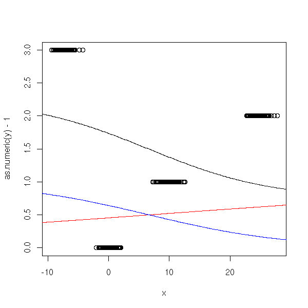
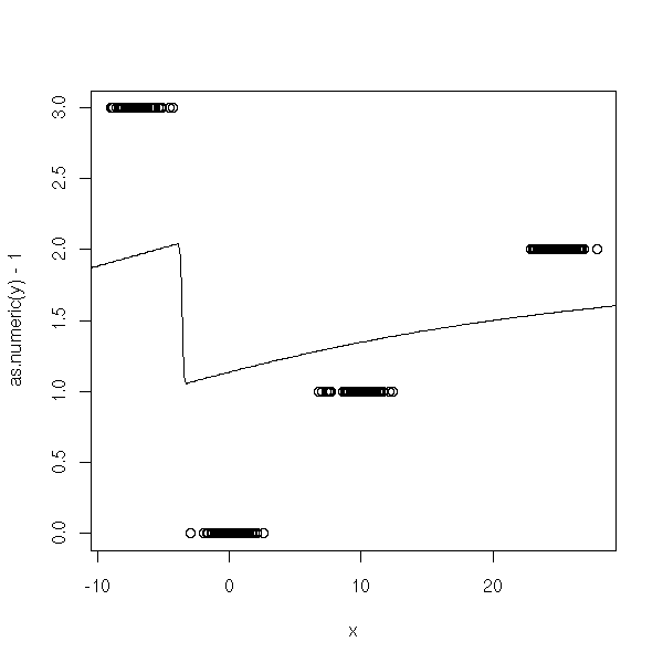
# NO!
n <- 100
x <- c( rnorm(n), 1+rnorm(n), 2.5+rnorm(n) )
y <- factor(c( rep(0,n), rep(1,n), rep(2,n) ))
r <- glm(y~x, family=binomial)
plot(as.numeric(y)-1~x)
xp <- seq(-5,5,length=200)
yp <- predict(r,data.frame(x=xp), type='response')
lines(xp,yp)
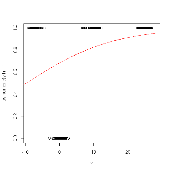
Let us try to encode the variable to predict with binary variables, by hand.
First attempt: brutally, thoughtlessly.
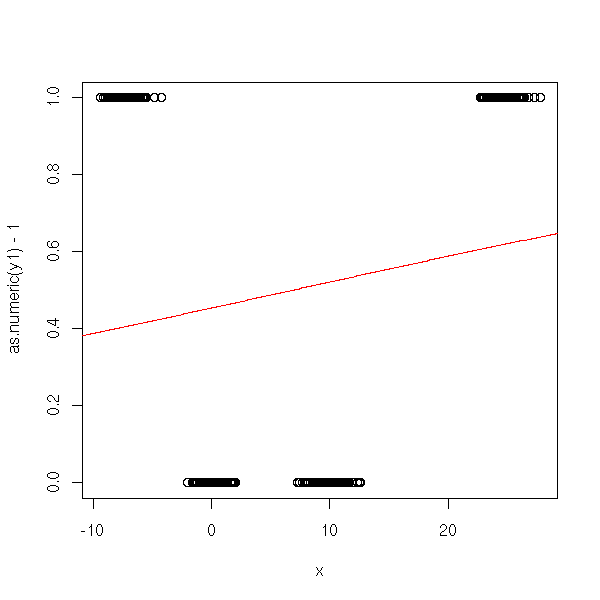
n <- 100
x <- c( rnorm(n), 10+rnorm(n), 25+rnorm(n), -7 + rnorm(n) )
y <- factor(c( rep(0,n), rep(1,n), rep(2,n), rep(3,n) ))
y1 <- factor(c( rep(0,n), rep(0,n), rep(1,n), rep(1,n) ))
y2 <- factor(c( rep(0,n), rep(1,n), rep(0,n), rep(1,n) ))
r1 <- glm(y1~x, family=binomial)
r2 <- glm(y2~x, family=binomial)
xp <- seq(-50,50,length=500)
y1p <- predict(r1,data.frame(x=xp), type='response')
y2p <- predict(r2,data.frame(x=xp), type='response')

plot(as.numeric(y)-1~x)
lines(xp,y1p+2*y2p)
lines(xp,y1p, col='red')
lines(xp,y2p, col='blue')
It does not workm because Y1 and Y2 do not come from a logistic model:
plot(as.numeric(y1)-1~x)
lines(xp,y1p, col='red')
Second attempt.
n <- 100
x <- c( rnorm(n), 10+rnorm(n), 25+rnorm(n), -7 + rnorm(n) )
y <- factor(c( rep(0,n), rep(1,n), rep(2,n), rep(3,n) ))
y1 <- factor(c( rep(0,n), rep(1,n), rep(1,n), rep(1,n) ))
y2 <- factor(c( rep(0,n), rep(0,n), rep(1,n), rep(1,n) ))
y3 <- factor(c( rep(0,n), rep(0,n), rep(0,n), rep(1,n) ))
r1 <- glm(y1~x, family=binomial)
r2 <- glm(y2~x, family=binomial)
r3 <- glm(y3~x, family=binomial)
xp <- seq(-50,50,length=500)
y1p <- predict(r1,data.frame(x=xp), type='response')
y2p <- predict(r2,data.frame(x=xp), type='response')
y3p <- predict(r3,data.frame(x=xp), type='response')

plot(as.numeric(y)-1~x)
lines(xp,y1p+y2p+y3p)
Same problem...
plot(as.numeric(y1)-1~x)
lines(xp,y1p, col='red')
Third attempt: with ordinal variables.
n <- 100
x <- c( -7+rnorm(n), rnorm(n), 10+rnorm(n), 25+rnorm(n))
y <- factor(c( rep(0,n), rep(1,n), rep(2,n), rep(3,n) ))
y1 <- factor(c( rep(0,n), rep(1,n), rep(1,n), rep(1,n) ))
y2 <- factor(c( rep(0,n), rep(0,n), rep(1,n), rep(1,n) ))
y3 <- factor(c( rep(0,n), rep(0,n), rep(0,n), rep(1,n) ))
r1 <- glm(y1~x, family=binomial)
r2 <- glm(y2~x, family=binomial)
r3 <- glm(y3~x, family=binomial)
xp <- seq(-50,50,length=500)
y1p <- predict(r1,data.frame(x=xp), type='response')
y2p <- predict(r2,data.frame(x=xp), type='response')
y3p <- predict(r3,data.frame(x=xp), type='response')

plot(as.numeric(y)-1~x)
lines(xp,y1p+y2p+y3p)
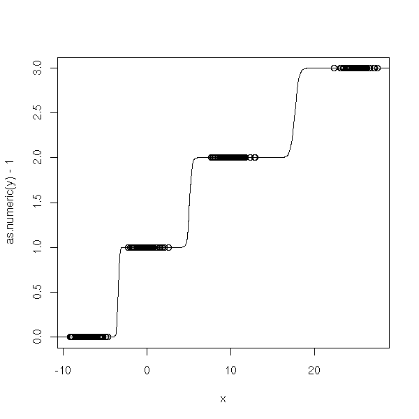
n <- 100
x <- c( -.7+rnorm(n), rnorm(n), 1+rnorm(n), 2.5+rnorm(n))
y <- factor(c( rep(0,n), rep(1,n), rep(2,n), rep(3,n) ))
y1 <- factor(c( rep(0,n), rep(1,n), rep(1,n), rep(1,n) ))
y2 <- factor(c( rep(0,n), rep(0,n), rep(1,n), rep(1,n) ))
y3 <- factor(c( rep(0,n), rep(0,n), rep(0,n), rep(1,n) ))
r1 <- glm(y1~x, family=binomial)
r2 <- glm(y2~x, family=binomial)
r3 <- glm(y3~x, family=binomial)
xp <- seq(-5,5,length=500)
y1p <- predict(r1,data.frame(x=xp), type='response')
y2p <- predict(r2,data.frame(x=xp), type='response')
y3p <- predict(r3,data.frame(x=xp), type='response')

plot(as.numeric(y)-1~x)
lines(xp,y1p+y2p+y3p)
lines(xp,round(y1p+y2p+y3p, digits=0), col='red')
You can also use logistic regression to forecast an ordinal qualitative variable (i.e., a qualitative variable whose values are ordered, -- e.g., its values could be "low", "medium", "high"). Here are some of the models you might want to use.
Proportionnal odds model (the effects are monotonic with respect to the quantitative variable):
                            1
P[ Y >= j | X ] = -----------------------
                         - ( a_j + X b )
                   1 + e
Continuation ratio model:
                                    1
P [ Y = j | Y >= j, X ] = -----------------------
                                - ( a_j + X b )
                           1 + e
Actually, our attempts in the preceding paragraph have led us to the first model.
n <- 100
x <- c( -.7+rnorm(n), rnorm(n), 1+rnorm(n), 2.5+rnorm(n))
y <- factor(c( rep(0,n), rep(1,n), rep(2,n), rep(3,n) ))
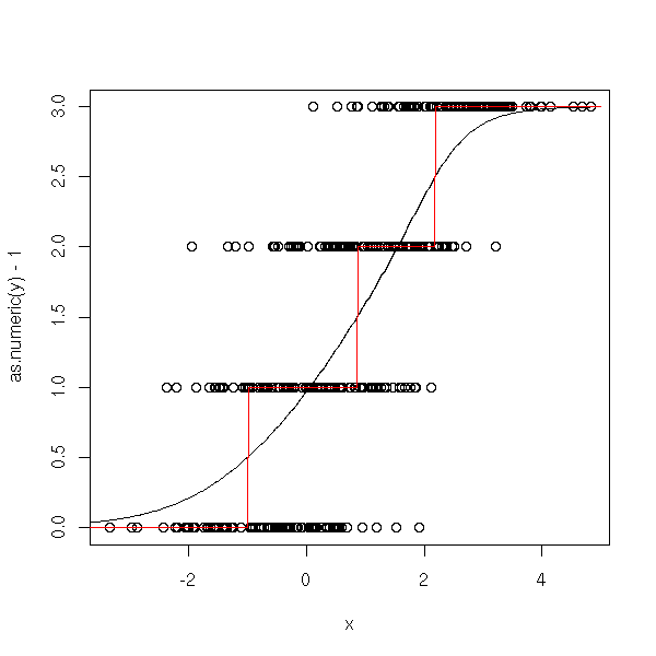
ordinal.regression.one <- function (y,x) {
xp <- seq(min(x),max(x), length=100)
yi <- matrix(nc=length(levels(y)), nr=length(y))
ri <- list();
ypi <- matrix(nc=length(levels(y)), nr=100)
for (i in 1:length(levels(y))) {
yi[,i] <- as.numeric(y) >= i
ri[[i]] <- glm(yi[,i] ~ x, family=binomial)
ypi[,i] <- predict(ri[[i]], data.frame(x=xp), type='response')
}
plot(as.numeric(y) ~ x)
lines(xp, apply(ypi,1,sum), col='red', lwd=3)
}
ordinal.regression.one(y,x)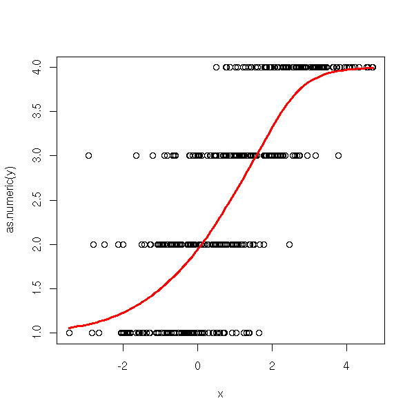
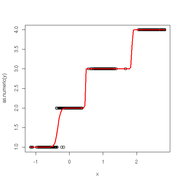
n <- 100
v <- .2
x <- c( -.7+v*rnorm(n), v*rnorm(n), 1+v*rnorm(n), 2.5+v*rnorm(n))
y <- factor(c( rep(0,n), rep(1,n), rep(2,n), rep(3,n) ))
ordinal.regression.one(y,x)
Here is the second.
n <- 100
x <- c( -.7+rnorm(n), rnorm(n), 1+rnorm(n), 2.5+rnorm(n))
y <- factor(c( rep(0,n), rep(1,n), rep(2,n), rep(3,n) ))
ordinal.regression.two <- function (y,x) {
  xp <- seq(min(x),max(x), length=100)
  yi <- list();
  ri <- list();
  ypi <- matrix(nc=length(levels(y)), nr=100)
  for (i in 1:length(levels(y))) {
    ya <- as.numeric(y)
    o <- ya >= i
    ya <- ya[o]
    xa <- x[o]
    yi[[i]] <- ya == i
    ri[[i]] <- glm(yi[[i]] ~ xa, family=binomial)
    ypi[,i] <- predict(ri[[i]], data.frame(xa=xp), type='response')
  }

  # The plot is trickier to draw than earlier
  plot(as.numeric(y) ~ x)
  p <- matrix(0, nc=length(levels(y)), nr=100)
  for (i in 1:length(levels(y))) {
    p[,i] = ypi[,i] * (1 - apply(p,1,sum))
  }
  for (i in 1:length(levels(y))) {
    p[,i] = p[,i]*i
  }
  lines(xp, apply(p,1,sum), col='red', lwd=3)
}
ordinal.regression.two(y,x)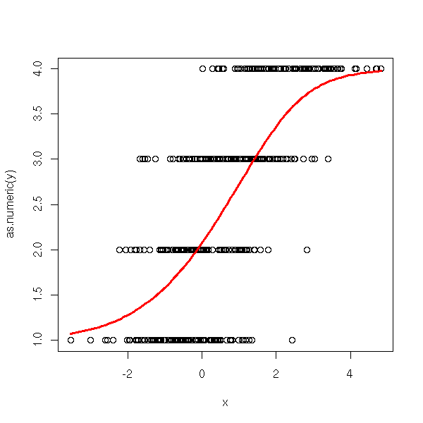
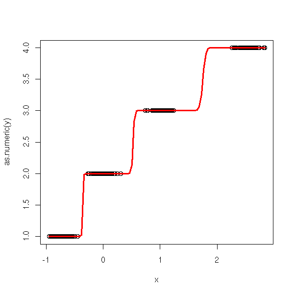
n <- 100
v <- .1
x <- c( -.7+v*rnorm(n), v*rnorm(n), 1+v*rnorm(n), 2.5+v*rnorm(n))
y <- factor(c( rep(0,n), rep(1,n), rep(2,n), rep(3,n) ))
ordinal.regression.two(y,x)
Actually, it is already implemented:
library(MASS)
?polr
We want to predict a qualitative variable, with more tham two values.
TODO
Model:
     P( Y=1 | X=x )
log ---------------- = b_{1,0} + b_1 x
     P( Y=k | X=x )

     P( Y=2 | X=x )
log ---------------- = b_{2,0} + b_2 x
     P( Y=k | X=x )

     P( Y=k-1 | X=x )
log ------------------ = b_{k-1,0} + b_{k-1} x
      P( Y=k | X=x )

(fit with MLE)

library(nnet)
?multinom

If the variable is binary, we get the same results as with a
classical logistic regression -- TODO: check this.

This work is licensed under a Creative Commons Attribution-NonCommercial-ShareAlike 2.5 License.
Vincent Zoonekynd
<zoonek@math.jussieu.fr>
latest modification on Sat Jan 6 10:28:22 GMT 2007