
Tests and confidence intervals
Partial residual plots, added variable plots
Some plots to explore a regression
Overfit
Underfit
Influential points
Influential clusters
Non gaussian residuals
Heteroskedasticity
Correlated errors
Unidentifiability
Missing values
Extrapolation
Miscellaneous
The curse of dimension
Wide problems
In this chapter, we list some of the problems that may occur in a regression and explain how to spot them -- graphically. Often, you can solve the problem by transforming the variables (so that the outliers and influential observations disappear, so that the residuals look normal, so that the residuals have the same variance -- quite often, you can do all this at the same time), by altering the model (for a simpler or more complex one) or by using another regression (GLS to account for heteroskedasticity and correlated residuals, robust regression to account for remaining influencial observations).
Overfit: choose a simpler model
Underfit: curvilinear regression, non-linear regression, local regression
Influential points: transform the data, robust regression, weighted
                    least squares, remove the points
Influential clusters: transform the data, mixtures
Non-gaussian residuals: transform the data, robust regression, normalp
Heteroskedasticity: gls
correlated residuals: gls
Unidentifiability: shrinkage methods
Missing values: discard the observations???
The curse of dimension (GAM,...)
Combining regressions (BMA,...)
After this bird's eye view of several regression techniques, let us come back to linear regression.
The "summary" function gave us the results of a Student T test on the regression coefficients -- that answered the question "is this coefficient significantly different from zero?".
> x <- rnorm(100)
> y <- 1 + 2*x + .3*rnorm(100)
> summary(lm(y~x))
...
Coefficients:
            Estimate Std. Error t value Pr(>|t|)
(Intercept)  1.08440    0.03224   33.64   <2e-16 ***
x            2.04051    0.03027   67.42   <2e-16 ***
In the same example, if we have a prior idea on the value of the coefficient, we can test this value: here, let us test if the intercept is 1.
(When you write a formula to describe a model, some operators are interpreted in a different way (especially * and ^): to be sure that they will be understood as arithmetic operations on the variables, surround them with I(...). Here, it is not needed.)
> x <- rnorm(100)
> y <- 1 + 2*x + .3*rnorm(100)
> summary(lm(I(y-1)~x))

Call:
lm(formula = I(y - 1) ~ x)

Residuals:
     Min       1Q   Median       3Q      Max
-0.84692 -0.24891  0.02781  0.20486  0.60522

Coefficients:
            Estimate Std. Error t value Pr(>|t|)
(Intercept) -0.01294    0.02856  -0.453    0.651
x            1.96405    0.02851  68.898   <2e-16 ***
---
Signif. codes:  0 `***' 0.001 `**' 0.01 `*' 0.05 `.' 0.1 ` ' 1

Residual standard error: 0.2855 on 98 degrees of freedom
Multiple R-Squared: 0.9798,     Adjusted R-squared: 0.9796
F-statistic:  4747 on 1 and 98 DF,  p-value: < 2.2e-16
Under the hypothesis that this coefficient is 1, let us check if the other is zero.
> summary(lm(I(y-1)~0+x))

Call:
lm(formula = I(y - 1) ~ 0 + x)

Residuals:
     Min       1Q   Median       3Q      Max
-0.85962 -0.26189  0.01480  0.19184  0.59227

Coefficients:
  Estimate Std. Error t value Pr(>|t|)
x  1.96378    0.02839   69.18   <2e-16 ***
---
Signif. codes:  0 `***' 0.001 `**' 0.01 `*' 0.05 `.' 0.1 ` ' 1

Residual standard error: 0.2844 on 99 degrees of freedom
Multiple R-Squared: 0.9797,     Adjusted R-squared: 0.9795
F-statistic:  4786 on 1 and 99 DF,  p-value: < 2.2e-16
Other method:
> x <- rnorm(100)
> y <- 1 + 2*x + .3*rnorm(100)
> a <- rep(1,length(x))
> summary(lm(y~offset(a)-1+x))

Call:
lm(formula = y ~ offset(a) - 1 + x)

Residuals:
     Min       1Q   Median       3Q      Max
-0.92812 -0.09901  0.09515  0.28893  0.99363

Coefficients:
  Estimate Std. Error t value Pr(>|t|)
x  2.04219    0.03114   65.58   <2e-16 ***
---
Signif. codes:  0 `***' 0.001 `**' 0.01 `*' 0.05 `.' 0.1 ` ' 1

Residual standard error: 0.3317 on 99 degrees of freedom
Multiple R-Squared: 0.9816,     Adjusted R-squared: 0.9815
F-statistic:  5293 on 1 and 99 DF,  p-value: < 2.2e-16
Let us check if it is equal to 2:
> summary(lm(I(y-1-2*x)~0+x))

Call:
lm(formula = I(y - 1 - 2 * x) ~ 0 + x)

Residuals:
     Min       1Q   Median       3Q      Max
-0.85962 -0.26189  0.01480  0.19184  0.59227

Coefficients:
  Estimate Std. Error t value Pr(>|t|)
x -0.03622    0.02839  -1.276    0.205

Residual standard error: 0.2844 on 99 degrees of freedom
Multiple R-Squared: 0.01618,    Adjusted R-squared: 0.006244
F-statistic: 1.628 on 1 and 99 DF,  p-value: 0.2049
Other method:
> summary(lm(y~offset(1+2*x)+0+x))
Call:
lm(formula = y ~ offset(1 + 2 * x) + 0 + x)

Residuals:
     Min       1Q   Median       3Q      Max
-0.92812 -0.09901  0.09515  0.28893  0.99363

Coefficients:
  Estimate Std. Error t value Pr(>|t|)
x  0.04219    0.03114   1.355    0.179

Residual standard error: 0.3317 on 99 degrees of freedom
Multiple R-Squared: 0.9816,     Adjusted R-squared: 0.9815
F-statistic:  5293 on 1 and 99 DF,  p-value: < 2.2e-16
More generally, you can use the "offset" function in a linear regression when you know exactly one of the coefficients.
Other method:
x <- rnorm(100)
y <- 1 + 2*x + .3*rnorm(100)
library(car)
linear.hypothesis( lm(y~x), matrix(c(1,0,0,1), 2, 2), c(1,2) )
This checks if
[ 1  0 ]   [ first coefficient  ]   [ 1 ]
[      ] * [                    ] = [   ]
[ 0  1 ]   [ second coefficient ]   [ 2 ].
This yields:
F-Test
SS = 0.04165324     SSE = 9.724817     F = 0.2098763  Df = 2 and 98     p = 0.8110479
You can compute confidence intervals on the parameters.
> library(MASS)
> n <- 100
> x <- rnorm(n)
> y <- 1 - 2*x + rnorm(n)
> r <- lm(y~x)
> r$coefficients
(Intercept)           x
  0.9569173  -2.1296830
> confint(r)
                 2.5 %    97.5 %
(Intercept)  0.7622321  1.151603
x           -2.3023449 -1.957021
You can also look for confidence intervals on the predicted values. It can be a confidence interval of aX+b (confidence band) or -- this is different -- of E[Y|X=x] (prediction band).
x <- runif(20)
y <- 1-2*x+.1*rnorm(20)
res <- lm(y~x)
plot(y~x)
new <- data.frame( x=seq(0,1,length=21) )
p <- predict(res, new)
points( p ~ new$x, type='l' )
p <- predict(res, new, interval='confidence')
points( p[,2] ~ new$x, type='l', col="green" )
points( p[,3] ~ new$x, type='l', col="green" )
p <- predict(res, new, interval='prediction')
points( p[,2] ~ new$x, type='l', col="red" )
points( p[,3] ~ new$x, type='l', col="red" )
title(main="Confidence and prediction bands")
legend( par("usr")[1], par("usr")[3], yjust=0,
        c("Confidence band", "Prediction band"),
        lwd=1, lty=1, col=c("green", "red") )
TODO: stress the difference between the two...
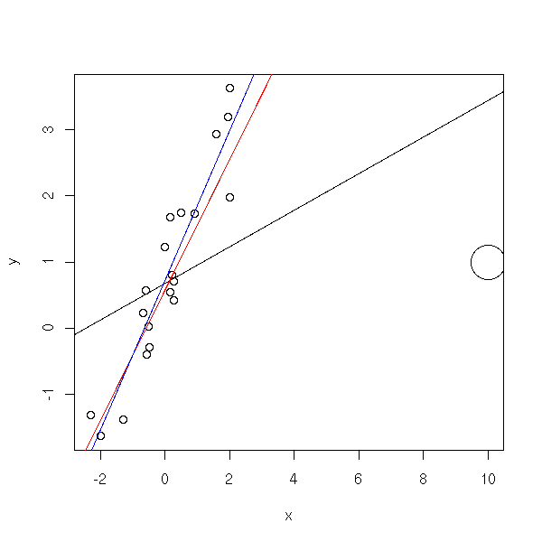
Away from the values of the sample, the intervals grow.
plot(y~x, xlim=c(-1,2), ylim=c(-3,3))
new <- data.frame( x=seq(-2,3,length=200) )
p <- predict(res, new)
points( p ~ new$x, type='l' )
p <- predict(res, new, interval='confidence')
points( p[,2] ~ new$x, type='l', col="green" )
points( p[,3] ~ new$x, type='l', col="green" )
p <- predict(res, new, interval='prediction')
points( p[,2] ~ new$x, type='l', col="red" )
points( p[,3] ~ new$x, type='l', col="red" )
title(main="Confidence and prediction bands")
legend( par("usr")[1], par("usr")[3], yjust=0,
        c("Confidence band", "Prediction band"),
        lwd=1, lty=1, col=c("green", "red") )
plot(y~x, xlim=c(-5,6), ylim=c(-11,11))
new <- data.frame( x=seq(-5,6,length=200) )
p <- predict(res, new)
points( p ~ new$x, type='l' )
p <- predict(res, new, interval='confidence')
points( p[,2] ~ new$x, type='l', col="green" )
points( p[,3] ~ new$x, type='l', col="green" )
p <- predict(res, new, interval='prediction')
points( p[,2] ~ new$x, type='l', col="red" )
points( p[,3] ~ new$x, type='l', col="red" )
title(main="Confidence and prediction bands")
legend( par("usr")[1], par("usr")[3], yjust=0,
        c("Confidence band", "Prediction band"),
        lwd=1, lty=1, col=c("green", "red") )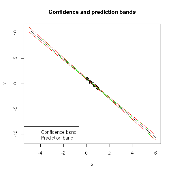
Here are other ways of representing the confidence and prediction intervals.
N <- 100
n <- 20
x <- runif(N, min=-1, max=1)
y <- 1 - 2*x + rnorm(N, sd=abs(x))
res <- lm(y~x)
plot(y~x)
x0 <- seq(-1,1,length=n)
new <- data.frame( x=x0 )
p <- predict(res, new)
points( p ~ x0, type='l' )
p <- predict(res, new, interval='prediction')
segments( x0, p[,2], x0, p[,3], col='red')
p <- predict(res, new, interval='confidence')
segments( x0, p[,2], x0, p[,3], col='green', lwd=3 )

mySegments <- function(a,b,c,d,...) {
  u <- par('usr')
  e <- (u[2]-u[1])/100
  segments(a,b,c,d,...)
  segments(a+e,b,a-e,b,...)
  segments(c+e,d,c-e,d,...)
}
plot(y~x)
p <- predict(res, new)
points( p ~ x0, type='l' )
p <- predict(res, new, interval='prediction')
mySegments( x0, p[,2], x0, p[,3], col='red')
p <- predict(res, new, interval='confidence')
mySegments( x0, p[,2], x0, p[,3], col='green', lwd=3 )
You can want a confidence interval for a single, isolated, parameter -- you get an interval -- or for several parameters at a time -- you get an ellipsoid, called the confidence region. It brings more information than the 1-variable confidence intervals (you cannot combine those intervals). Thus you might want to plot these ellipses.
The ellipse you get is skewed, because it comes from the correlation matrix of the two coefficients: simply diagonalize it in an orthonormal basis and the eigen vectors will give you the axes.
library(ellipse)
my.confidence.region <- function (g, a=2, b=3) {
  e <- ellipse(g,c(a,b))
  plot(e,
       type="l",
       xlim=c( min(c(0,e[,1])), max(c(0,e[,1])) ),
       ylim=c( min(c(0,e[,2])), max(c(0,e[,2])) ),
      )
  x <- g$coef[a]
  y <- g$coef[b]
  points(x,y,pch=18)
  cf <- summary(g)$coefficients
  ia <- cf[a,2]*qt(.975,g$df.residual)
  ib <- cf[b,2]*qt(.975,g$df.residual)
  abline(v=c(x+ia,x-ia),lty=2)
  abline(h=c(y+ib,y-ib),lty=2)
  points(0,0)
  abline(v=0,lty="F848")
  abline(h=0,lty="F848")
}

n <- 20
x1 <- rnorm(n)
x2 <- rnorm(n)
x3 <- rnorm(n)
y <- x1+x2+x3+rnorm(n)
g <- lm(y~x1+x2+x3)
my.confidence.region(g)
n <- 20
x <- rnorm(n)
x1 <- x+.2*rnorm(n)
x2 <- x+.2*rnorm(n)
y <- x1+x2+rnorm(n)
g <- lm(y~x1+x2)
my.confidence.region(g)
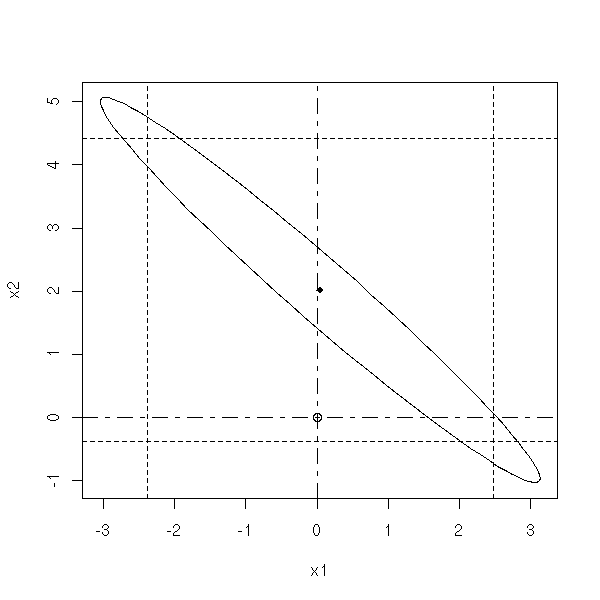
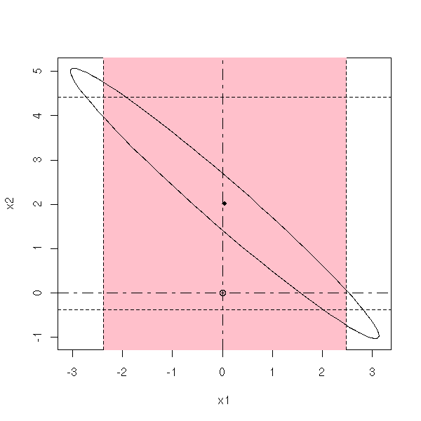
In the three following plots, the probability that the actual values of the parameters be in the pink area is the same.
my.confidence.region <- function (g, a=2, b=3, which=0, col='pink') {
  e <- ellipse(g,c(a,b))
  x <- g$coef[a]
  y <- g$coef[b]
  cf <- summary(g)$coefficients
  ia <- cf[a,2]*qt(.975,g$df.residual)
  ib <- cf[b,2]*qt(.975,g$df.residual)
  xmin <- min(c(0,e[,1]))
  xmax <- max(c(0,e[,1]))
  ymin <- min(c(0,e[,2]))
  ymax <- max(c(0,e[,2]))
  plot(e,
       type="l",
       xlim=c(xmin,xmax),
       ylim=c(ymin,ymax),
      )
  if(which==1){ polygon(e,col=col) }
  else if(which==2){ rect(x-ia,par('usr')[3],x+ia,par('usr')[4],col=col,border=col) }
  else if(which==3){ rect(par('usr')[1],y-ib,par('usr')[2],y+ib,col=col,border=col) }
  lines(e)
  points(x,y,pch=18)
  abline(v=c(x+ia,x-ia),lty=2)
  abline(h=c(y+ib,y-ib),lty=2)
  points(0,0)
  abline(v=0,lty="F848")
  abline(h=0,lty="F848")
}
my.confidence.region(g, which=1)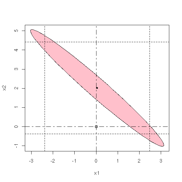
my.confidence.region(g, which=2)
my.confidence.region(g, which=3)

When you perform a multiple regression, you try to retain as few predictive variables as possible, while retaining all those that are relevant. To choose or discard variables, you might be tempted to perform a lot of statistical tests.
This is a bad idea.
Indeed, for each testm you have a certain risk of making a mistake -- and those risks pile up.
However, this is usually what we do -- we rarely have the choice. You can either start with a model with no variable at all, then add the "best" predictive variable (say, the one with the higher correlation) and progressively add other variables (say, the ones that provide the biggest increase in R^2) and stop when you reach a certain criterion (say, when F^2 reaches a certain value); or start with a saturated model, containing all the variables an successively remove the variables that provide the smallest decrease in R^2 and stop when F^2 reaches a value fixed in advance.
TODO: Tukey, etc. (in the Anova chapter?)
When you read regression or anova (analysis of variance) results, you often face a table "full of sums of squares".
RSS (Residual Sum of Squares): this is the quantity you try to minimize in a regression. More precisely, let X be the predictive variable, Y the variable to predict and hat(Yi) the predicted velue, we set
hat Yi = b0 + b1 Xi
and we try to find the values of b0 and b1 that minimize
RSS = Sum( (Yi - hat Yi)^2 ).
TSS (Total sum of squares): The is the sun of squares minimized when you look for the mean of Y
TSS = Sum( (Yi - bar Y)^2 )
ESS (Explained Sum of Squares): This is the difference between the preceding two sums of squares. It can also be written as a sum of squares.
ESS = Sum( ( hat Yi - bar Y )^2 )
R-square: "determination coefficient" or "percentage of variance of Y explained by X". The closer to one, the better the regression explains the variations of Y.
R^2 = ESS/TSS.
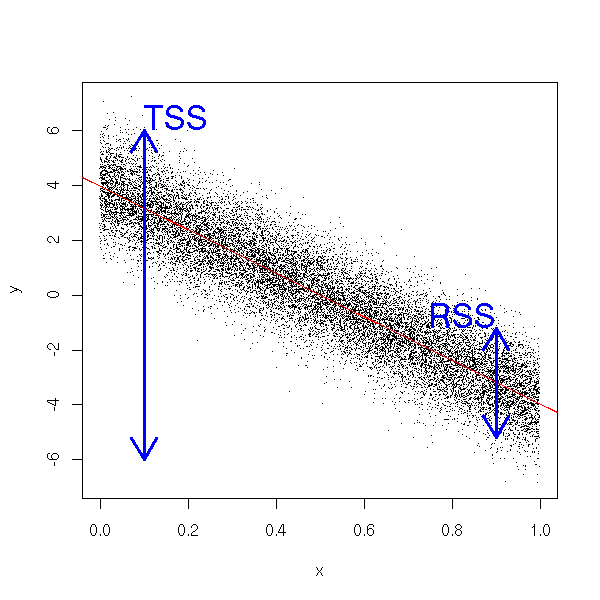
You can give a graphical interpretation of the determination coefficient. The data are clustered in a band of height RSS around the regression line, while the height of the plot is TSS. We then have R^2=1-RSS/TSS.
n <- 20000
x <- runif(n)
y <- 4 - 8*x + rnorm(n)
plot(y~x, pch='.')
abline(lm(y~x), col='red')
arrows( .1, -6, .1, 6, code=3, lwd=3, col='blue' )
arrows( .9, -3.2-2, .9, -3.2+2, code=3, lwd=3, col='blue' )
text( .1, 6, "TSS", adj=c(0,0), cex=2, col='blue' )
text( .9, -3.2+2, "RSS", adj=c(1,0), cex=2, col='blue' )
We have seen three way of printing the results of a regression: with the "print", "summary" and "anova" functions. The last line of the "anova" function compares our model with the null model (i.e., with the model with no explanatory variables at all, y ~ 1).
> x <- rnorm(100)
> y <- 1 + 2*x + .3*rnorm(100)
> summary(lm(y~x))

Call:
lm(formula = y ~ x)

Residuals:
     Min       1Q   Median       3Q      Max
-0.84692 -0.24891  0.02781  0.20486  0.60522

Coefficients:
            Estimate Std. Error t value Pr(>|t|)
(Intercept)  0.98706    0.02856   34.56   <2e-16 ***
x            1.96405    0.02851   68.90   <2e-16 ***
---
Signif. codes:  0 `***' 0.001 `**' 0.01 `*' 0.05 `.' 0.1 ` ' 1

Residual standard error: 0.2855 on 98 degrees of freedom
Multiple R-Squared: 0.9798,     Adjusted R-squared: 0.9796
F-statistic:  4747 on 1 and 98 DF,  p-value: < 2.2e-16
The result of the "anova" function explains where these fugures come from: you have the sum of squares, their "mean" (just divide by the "number of degrees of freedom"), their quotient (F-value) and the probability that this quotient be as high if the slope of the line is zero (i.e., the p-value of the test of H0: "the slope is zero" against H1: "the slope is not zero").
> anova(lm(y~x))
Analysis of Variance Table

Response: y
          Df Sum Sq Mean Sq F value    Pr(>F)
x          1 386.97  386.97    4747 < 2.2e-16 ***
Residuals 98   7.99    0.08
---
Signif. codes:  0 `***' 0.001 `**' 0.01 `*' 0.05 `.' 0.1 ` ' 1
More generally, the "anova" function performs a test that compares embedded models (here, a model with an intercept and a slope, and a model with an intercept and no slope).
In a multiple regression, you strive to retain as few variables as possible. In this process, you want to compare models: e.g., compare a model with a lot of variable and a model with fewer variables.
The "anova" function performs that kind of comparison (it does not answer the question "is this model better?" but "are these models significantly different?" -- if they are not significantly different, you will reject the more complicated one).
data(trees)
r1 <- lm(Volume ~ Girth, data=trees)
r2 <- lm(Volume ~ Girth + Height, data=trees)
anova(r1,r2)
The result
Analysis of Variance Table

Model 1: Volume ~ Girth
Model 2: Volume ~ Girth + Height
  Res.Df    RSS Df Sum of Sq      F  Pr(>F)
1     29 524.30
2     28 421.92  1    102.38 6.7943 0.01449 *
---
Signif. codes:  0 `***' 0.001 `**' 0.01 `*' 0.05 `.' 0.1 ` ' 1
tells us that the two models are significantly different with a risk of error under 2%.
Here are a few other examples.
x1 <- rnorm(100)
x2 <- rnorm(100)
x3 <- rnorm(100)
b <- .1* rnorm(100)

y <- 1 + x1 + x2 + x3 + b
r1 <- lm( y ~ x1 )
r2 <- lm( y ~ x1 + x2 + x3 )
anova(r1,r2) # p-value = 2e-16

y <- 1 + x1
r1 <- lm( y ~ x1 )
r2 <- lm( y ~ x1 + x2 + x3 )
anova(r1,r2) # p-value = 0.25

y <- 1 + x1 + .02*x2 - .02*x3 + b
r1 <- lm( y ~ x1 )
r2 <- lm( y ~ x1 + x2 + x3 )
anova(r1,r2) # p-value = 0.10
You can compare more that two model (but always nested models: each model is included in the next).
y <- 1 + x1 + x2 + x3 + b
r1 <- lm( y ~ x1 )
r2 <- lm( y ~ x1 + x2 )
r3 <- lm( y ~ x1 + x2 + x3 )
anova(r1,r2,r3) # p-values = 2e-16 (both)
If, in the comparison of two models, you get a very high p-value, i.e., if the two models are not significantly different, you will reject the more complex and retain the simplest.
You can present the computations performed in a regression as an anova table. Furthermore, the idea behind the computations is the same: express the variance of Y as the sum of a variance of a variable affine in X and a residual variance, and minimize this residual variance.
x <- runif(10)
y <- 1 + x + .2*rnorm(10)
anova(lm(y~x))
Here, the anova tells us that, indeed, Y depend on X, with a risk of error under 1%.
Analysis of Variance Table

Response: y
          Df  Sum Sq Mean Sq F value   Pr(>F)
x          1 0.85633 0.85633  20.258 0.002000 **
Residuals  8 0.33817 0.04227
It still works with several predictive variables.
x <- runif(10)
y <- runif(10)
z <- 1 + x - y + .2*rnorm(10)
anova(lm(z~x+y))
The analysis of variance table tells us that z depends on x and y, with a risk of error under 1%.
Analysis of Variance Table

Response: z
          Df  Sum Sq Mean Sq F value    Pr(>F)
x          1 2.33719 2.33719  45.294 0.0002699 ***
y          1 0.73721 0.73721  14.287 0.0068940 **
Residuals  7 0.36120 0.05160
Counterintuitive and frightening as it may be, you might notice that the result depends on the order of the parameters...
>   anova(lm(z~y+x))
Analysis of Variance Table

Response: z
          Df  Sum Sq Mean Sq F value   Pr(>F)
y          1 2.42444 2.42444  46.985 0.000241 ***
x          1 0.64996 0.64996  12.596 0.009355 **
Residuals  7 0.36120 0.05160
In some cases, you can even get contradictory results: depending on the order of the predictive variables, you can find that z sometimes depends on x, sometimes not.
> x <- runif(10)
> y <- runif(10)
> z <- 1 + x + 5*y + .2*rnorm(10)

> anova(lm(z~x+y))
Analysis of Variance Table
Response: z
          Df Sum Sq Mean Sq  F value    Pr(>F)
x          1 0.0104  0.0104   0.1402    0.7192
y          1 7.5763  7.5763 102.1495 1.994e-05 ***
Residuals  7 0.5192  0.0742

> anova(lm(z~y+x))
Analysis of Variance Table
Response: z
          Df Sum Sq Mean Sq F value    Pr(>F)
y          1 7.1666  7.1666  96.626 2.395e-05 ***
x          1 0.4201  0.4201   5.664   0.04889 *
Residuals  7 0.5192  0.0742
The residuals are the differences between the observed values and the predicted values.
The noise is the difference between the observed values and the actual values: it appears in the model, e.g.
Y = a + b X + noise
Residues and noise are two different things. Even from a statistical point of view, they look different. For instance, their variance is not the same (neither is the shape of their distribution, by the way). The following simulation estimates the variance of the residuals: we get 0.008893307 while the noise variance was 0.01.
a <- 1
b <- -2
s <- .1
n <- 10
N <- 1e6
v <- NULL
for (i in 1:N) {
  x <- rnorm(n)
  y <- 1-2*x+s*rnorm(n)
  v <- append(v, var(lm(y~x)$res))
}
mean(v)
You can show that the variance of the residual of the observation i is
sigma^2 * ( 1 - h_i )
where sigma^2 is the noise variance and h_i is the "leverage" of observation i (the i-th diagonal term of t(X)%*%X).
These are the normalized residuals. Their variance is estimated from all the sample.
?rstandard
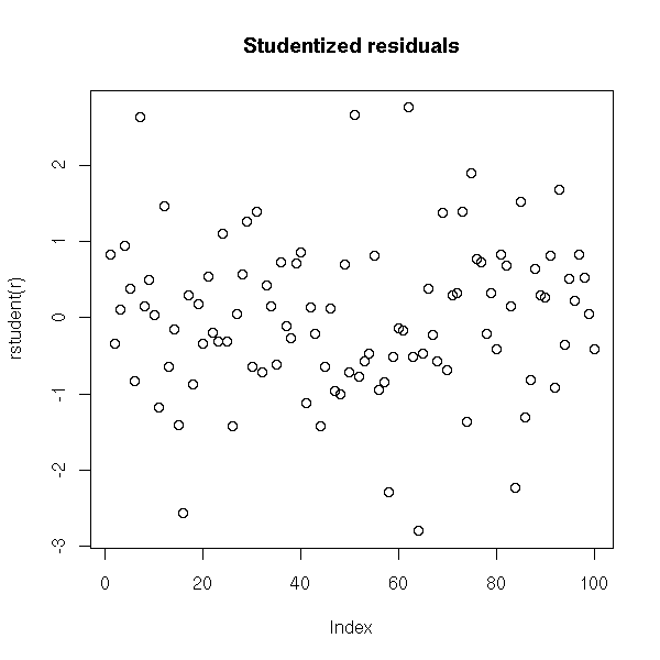
These are still the "normalized" residuals, but this time, we estimate the variance with the sample without the current observation.
?rstudent
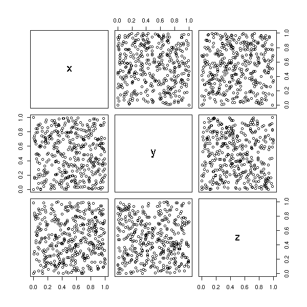
Let us consider the following example.
n <- 100
x1 <- rnorm(n)
x2 <- rnorm(n)
x3 <- x1^2+rnorm(n)
x4 <- 1/(1+x2^2)+.2*rnorm(n)
y <- 1+x1-x2+x3-x4+.1*rnorm(n)
pairs(cbind(x1,x2,x3,x4,y))

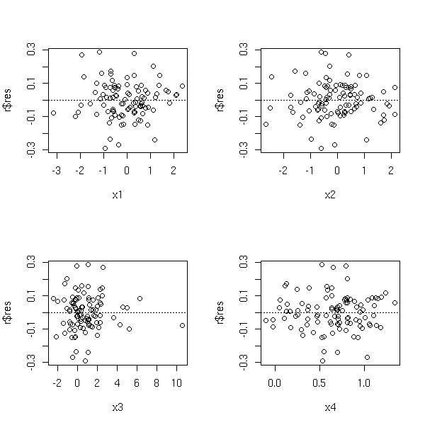
The residuals are full-fledged statistical variables: you can look at them through box-and-whisker plots, histograms, qqplots, etc. You can also plot them as a function of the predicted values, as a function of the various predictive variables or as a function of the observation number.
r <- lm(y~x1+x2+x3+x4)
boxplot(r$res, horizontal=T)

hist(r$res)

plot(r$res, main='Residuals')

plot(rstandard(r), main='Standardized residuals')

plot(rstudent(r), main="Studentized residuals")
plot(r$res ~ r$fitted.values,
     main="Residuals and predicted values")
abline(h=0, lty=3)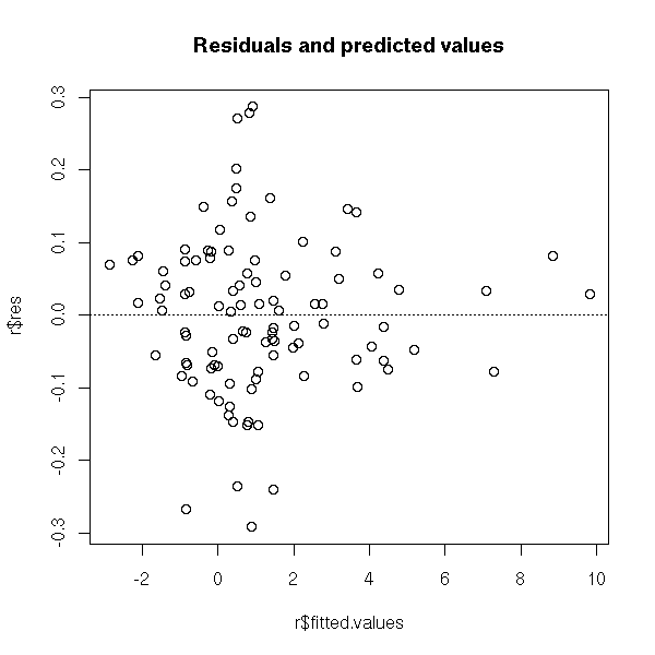
op <- par(mfrow=c(2,2))
plot(r$res ~ x1)
abline(h=0, lty=3)
plot(r$res ~ x2)
abline(h=0, lty=3)
plot(r$res ~ x3)
abline(h=0, lty=3)
plot(r$res ~ x4)
abline(h=0, lty=3)
par(op)
n <- 100
x1 <- rnorm(n)
x2 <- 1:n
y <- rnorm(1)
for (i in 2:n) {
  y <- c(y, y[i-1] + rnorm(1))
}
y <- x1 + y
r <- lm(y~x1+x2) # Or simply: lm(y~x1)
op <- par(mfrow=c(2,1))
plot( r$res ~ x1 )
plot( r$res ~ x2 )
par(op)
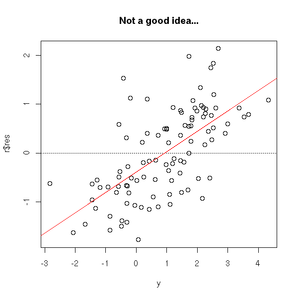
It is usually a bad idea to plot the residuals as a function of the observed values, because the "noise term" in the model appears on both axes, and you (almost) end up plotting this noise as a function of itself...
n <- 100
x <- rnorm(n)
y <- 1-x+rnorm(n)
r <- lm(y~x)
plot(r$res ~ y)
abline(h=0, lty=3)
abline(lm(r$res~y),col='red')
title(main='Not a good idea...')
Let us consider a regression situation with two predictive variables X1 and X2 and one variable to predict Y.
You can study the effect of X1 on Y after removing the (linear) effect of X2 on Y: simply regress Y against X2, X1 against X2 and plot the residuals of the former against those of the latter.
Those plots may help you spot influent observations.
partial.regression.plot <- function (y, x, n, ...) {
  m <- as.matrix(x[,-n])
  y1 <- lm(y ~ m)$res
  x1 <- lm(x[,n] ~ m)$res
  plot( y1 ~ x1, ... )
  abline(lm(y1~x1), col='red')
}

n <- 100
x1 <- rnorm(n)
x2 <- rnorm(n)
x3 <- x1+x2+rnorm(n)
x <- cbind(x1,x2,x3)
y <- x1+x2+x3+rnorm(n)
op <- par(mfrow=c(2,2))
partial.regression.plot(y, x, 1)
partial.regression.plot(y, x, 2)
partial.regression.plot(y, x, 3)
par(op)
There is already an "av.plot" function in the "car" package for this.
library(car)
av.plots(lm(y~x1+x2+x3),ask=F)

The "leverage.plots", still in the "car" package, generalizes this idea.
?leverage.plots
It is very similar to partial regression plots: this time, you plot Y, from which you have removed the effects of X2, as a function of X1. It is more efficient than oartial regression to spot non-linearities -- but partial regression is superior when it comes to spotting influent or outlying observations.
my.partial.residual.plot <- function (y, x, i, ...) {
  r <- lm(y~x)
  xi <- x[,i]
  # Y, minus the linear effects of X_j
  yi <- r$residuals + r$coefficients[i] * x[,i]
  plot( yi ~ xi, ... )
}
n <- 100
x1 <- rnorm(n)
x2 <- rnorm(n)
x3 <- x1+x2+rnorm(n)
x <- cbind(x1,x2,x3)
y <- x1+x2+x3+rnorm(n)
op <- par(mfrow=c(2,2))
my.partial.residual.plot(y, x, 1)
my.partial.residual.plot(y, x, 2)
my.partial.residual.plot(y, x, 3)
par(op)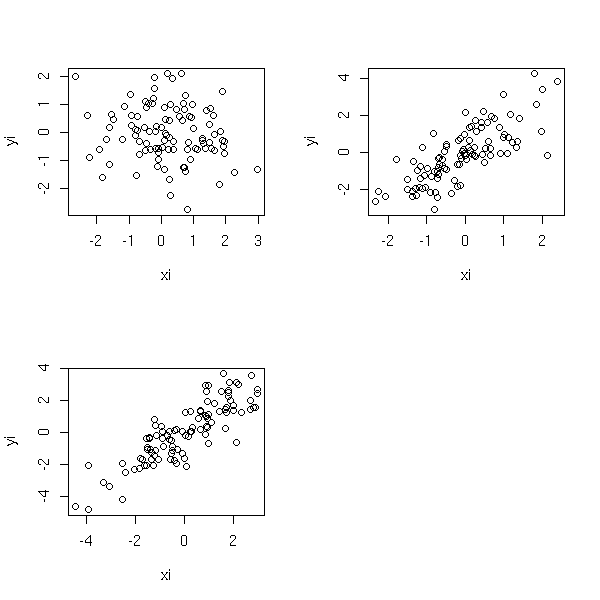
The "car" or "Design" packages provide functions to plot the partial residuals.
library(car)
?cr.plots
?ceres.plots

library(Design)
?plot.lrm.partial
?lrm
The regression might be "too close" to the data, to the point that it becomes irrealistic, that it performs poorly with "out-of-sample" data. The situation is not always as striking and obvious as here. However, if you want to choose, say, a non-linear model (or anyting complex), you must be able to justify it. In particular, compare the number of parameters to estimate with the number of observations...
n <- 10
x <- seq(0,1,length=n)
y <- 1-2*x+.3*rnorm(n)
plot(spline(x, y, n = 10*n), col = 'red', type='l', lwd=3)
points(y~x, pch=16, lwd=3, cex=2)
abline(lm(y~x))
title(main='Overfit')

This is mainly common-sense.
In the case of a linear regression, you can compare the determination coefficient (in case of overfit, it is close to 1) and the adjusted determination coefficient (that accounts for overfitting problems).
> summary(lm(y~poly(x,n-1)))
Call:
lm(formula = y ~ poly(x, n - 1))

Residuals:
ALL 10 residuals are 0: no residual degrees of freedom!

Coefficients:
                Estimate Std. Error t value Pr(>|t|)
(Intercept)      0.01196
poly(x, n - 1)1 -1.94091
poly(x, n - 1)2 -0.02303
poly(x, n - 1)3 -0.08663
poly(x, n - 1)4 -0.06938
poly(x, n - 1)5 -0.34501
poly(x, n - 1)6 -0.51048
poly(x, n - 1)7 -0.28479
poly(x, n - 1)8 -0.22273
poly(x, n - 1)9  0.39983

Residual standard error: NaN on 0 degrees of freedom
Multiple R-Squared:     1,      Adjusted R-squared:   NaN
F-statistic:   NaN on 9 and 0 DF,  p-value: NA

> summary(lm(y~poly(x,n-2)))
Call:
lm(formula = y ~ poly(x, n - 2))

Residuals:
        1         2         3         4         5         6         7         8         9        10
-0.001813  0.016320 -0.065278  0.152316 -0.228473  0.228473 -0.152316  0.065278 -0.016320  0.001813

Coefficients:
                Estimate Std. Error t value Pr(>|t|)
(Intercept)      0.01196    0.12644   0.095    0.940
poly(x, n - 2)1 -1.94091    0.39983  -4.854    0.129
poly(x, n - 2)2 -0.02303    0.39983  -0.058    0.963
poly(x, n - 2)3 -0.08663    0.39983  -0.217    0.864
poly(x, n - 2)4 -0.06938    0.39983  -0.174    0.891
poly(x, n - 2)5 -0.34501    0.39983  -0.863    0.547
poly(x, n - 2)6 -0.51048    0.39983  -1.277    0.423
poly(x, n - 2)7 -0.28479    0.39983  -0.712    0.606
poly(x, n - 2)8 -0.22273    0.39983  -0.557    0.676

Residual standard error: 0.3998 on 1 degrees of freedom
Multiple R-Squared: 0.9641,     Adjusted R-squared: 0.6767
F-statistic: 3.355 on 8 and 1 DF,  p-value: 0.4
If you are reasonable, the determination coefficient and its adjusted version are very close.
> x <- seq(0,1,length=n)
> y <- 1-2*x+.3*rnorm(n)
> summary(lm(y~poly(x,10)))

Call:
lm(formula = y ~ poly(x, 10))

Residuals:
      Min        1Q    Median        3Q       Max
-0.727537 -0.206951 -0.002332  0.177562  0.902353

Coefficients:
              Estimate Std. Error t value Pr(>|t|)
(Intercept)   -0.01312    0.02994  -0.438    0.662
poly(x, 10)1  -6.11784    0.29943 -20.431   <2e-16 ***
poly(x, 10)2  -0.11099    0.29943  -0.371    0.712
poly(x, 10)3  -0.04936    0.29943  -0.165    0.869
poly(x, 10)4  -0.28863    0.29943  -0.964    0.338
poly(x, 10)5  -0.15348    0.29943  -0.513    0.610
poly(x, 10)6   0.12146    0.29943   0.406    0.686
poly(x, 10)7   0.05066    0.29943   0.169    0.866
poly(x, 10)8   0.09707    0.29943   0.324    0.747
poly(x, 10)9   0.07554    0.29943   0.252    0.801
poly(x, 10)10  0.42494    0.29943   1.419    0.159
---
Signif. codes:  0 `***' 0.001 `**' 0.01 `*' 0.05 `.' 0.1 ` ' 1

Residual standard error: 0.2994 on 89 degrees of freedom
Multiple R-Squared: 0.8256,     Adjusted R-squared: 0.8059
F-statistic: 42.12 on 10 and 89 DF,  p-value: < 2.2e-16


> summary(lm(y~poly(x,1)))
...
Multiple R-Squared: 0.8182,     Adjusted R-squared: 0.8164
...
If the sample is too small, you will not be able to estimate much, In such situationm you have to restrict yourself to simple (simplistic) models, such as linear models, becaus the overfitting risk is too high.
TODO

Explain what you can do if there are more variables than
observations.
The naive approach will not work:
n <- 100
k <- 500
x <- matrix(rnorm(n*k), nr=n, nc=k)
y <- apply(x, 1, sum)
lm(y~x)

svm
Sometimes, the model is too simplistic.
x <- runif(100, -1, 1)
y <- 1-x+x^2+.3*rnorm(100)
plot(y~x)
abline(lm(y~x), col='red')

On the preceding plot, it is not obvious, but you can spot the problem if you try to see if a polynomial model would not be better,
> summary(lm(y~poly(x,10)))
...
Coefficients:
Estimate Std. Error t value Pr(>|t|)
(Intercept) 1.29896 0.02841 45.725 < 2e-16 ***
poly(x, 10)1 -4.98079 0.28408 -17.533 < 2e-16 ***
poly(x, 10)2 2.53642 0.28408 8.928 5.28e-14 ***
poly(x, 10)3 -0.06738 0.28408 -0.237 0.813
poly(x, 10)4 -0.15583 0.28408 -0.549 0.585
poly(x, 10)5 0.15112 0.28408 0.532 0.596
poly(x, 10)6 0.04512 0.28408 0.159 0.874
poly(x, 10)7 -0.29056 0.28408 -1.023 0.309
poly(x, 10)8 -0.39384 0.28408 -1.386 0.169
poly(x, 10)9 -0.25763 0.28408 -0.907 0.367
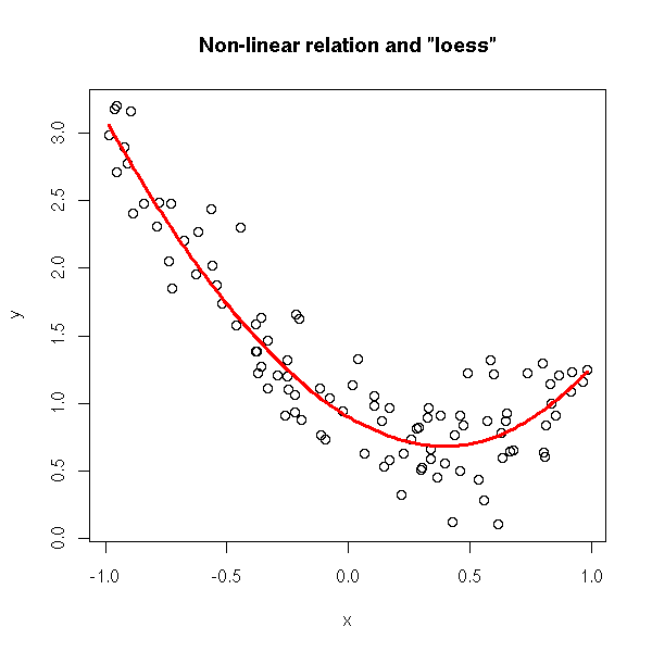
poly(x, 10)10 -0.09940 0.28408 -0.350 0.727or by using splines (or any other regularization method) an by looking at the result,
plot(y~x)
lines(smooth.spline(x,y), col='red', lwd=2)
title(main="Splines can help you spot non-linear relations")

plot(y~x)
lines(lowess(x,y), col='red', lwd=2)
title(main='Non-linear relations and "lowess"')

plot(y~x)
xx <- seq(min(x),max(x),length=100)
yy <- predict( loess(y~x), data.frame(x=xx) )
lines(xx,yy, col='red', lwd=3)
title(main='Non-linear relation and "loess"')
or by looking at the residuals with any regularization method (plot the residuals as a function of the predicted values or as a function of the predictive variables).
r <- lm(y~x)
plot(r$residuals ~ r$fitted.values,
      xlab='predicted values', ylab='residuals',
      main='Residuals and predicted values')
lines(lowess(r$fitted.values, r$residuals), col='red', lwd=2)
abline(h=0, lty=3)
plot(r$residuals ~ x,
      xlab='x', ylab='residuals',
      main='Residuals and the predictive variable')
lines(lowess(x, r$residuals), col='red', lwd=2)
abline(h=0, lty=3)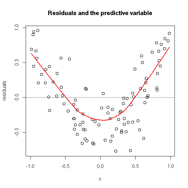
In some (rare) cases, you have several observations for the same value of the predictive variables: you can then perform the following test.
x <- rep(runif(10, -1, 1), 10)
y <- 1-x+x^2+.3*rnorm(100)
r1 <- lm(y ~ x)
r2 <- lm(y ~ factor(x))
anova(r1,r2)
Both models should give the same predictions: here, it is not the case.
Analysis of Variance Table

Model 1: y ~ x
Model 2: y ~ factor(x)
  Res.Df     RSS Df Sum of Sq      F    Pr(>F)
1     98 19.5259
2     90  6.9845  8   12.5414 20.201 < 2.2e-16 ***
---
Signif. codes:  0 `***' 0.001 `**' 0.01 `*' 0.05 `.' 0.1 ` ' 1
Let us try with a linear relation.
x <- rep(runif(10, -1, 1), 10)
y <- 1-x+.3*rnorm(100)
r1 <- lm(y ~ x)
r2 <- lm(y ~ factor(x))
anova(r1,r2)
The models are not significantly different.
Analysis of Variance Table

Model 1: y ~ x
Model 2: y ~ factor(x)
  Res.Df    RSS Df Sum of Sq      F Pr(>F)
1     98 9.6533
2     90 8.9801  8    0.6733 0.8435 0.5671
# Non-linearity
library(lmtest)
?harvtest
?raintest
?reset
The "strucchange" package detects structural changes (very often with time series, e.g., in econometry). There is a structural change when (for instance) the linear model is correct, but its coefficients change for time to time. If you know where the change occurs, you just split your sample into several chuks and perform a regression on each (to make sure that a change occured, you can test the equality of the coefficients in the chunks).
But usually, you do not know where the changes occur. You can try with moving window to find the most probable date for the structural change (you can take a window with a constant width, or one with a constrant number of observations).
TODO: an example

# Structural change
library(strucchange)
efp(..., type="Rec-CUSUM")
efp(..., type="OLS-MOSUM")
plot(efp(...))
sctest(efp(...))

TODO: an example

Fstat(...)
plot(Fstat(...))
sctest(Fstat(...))
Some points might bear an abnormally high influence on the regression results. SOmetimes, they come from mistakes (they should be identified and corrected), sometimes, they are perfectly normal but extreme. The leverage effect can yield incorrect results.
n <- 20
done.outer <- F
while (!done.outer) {
done <- F
while(!done) {
x <- rnorm(n)
done <- max(x)>4.5
}
y <- 1 - 2*x + x*rnorm(n)
r <- lm(y~x)
done.outer <- max(cooks.distance(r))>5
}
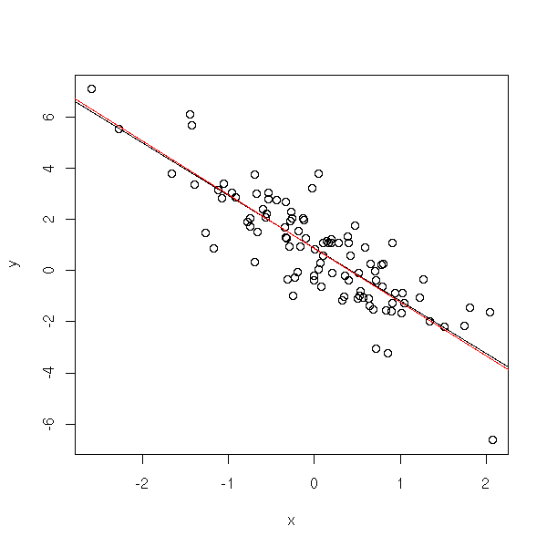
plot(y~x)
abline(1,-2,lty=2)
abline(lm(y~x),col='red',lwd=3)
lm(y~x)$coef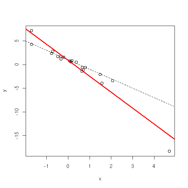
The first thing to do, even before starting the regression, is to look at the variables one at a time.
boxplot(x, horizontal=T)

stripchart(x, method='jitter')

hist(x, col='light blue', probability=T)
lines(density(x), col='red', lwd=3)

Same for y.
boxplot(y, horizontal=T)
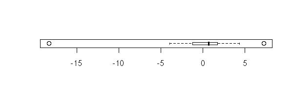
stripchart(y, method='jitter')

hist(y, col='light blue', probability=T)
lines(density(y), col='red', lwd=3)
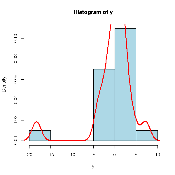
Here, there is an extreme point. AS there is a single one, we might be tempted to remove it -- if there were several, we would rather try to transform the data.
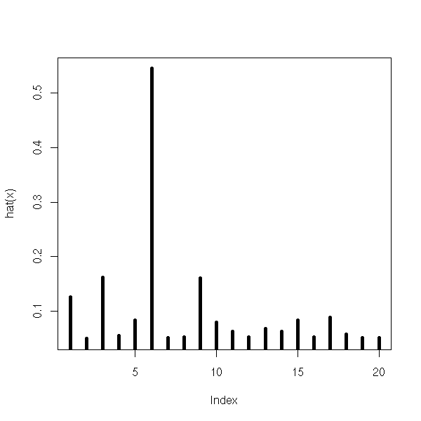
There is a measure of the "extremeness" of a point -- its leverage --: the diagonal elements of the hat matrix
H = X (X' X)^-1 X'
It is called "hat matrix" because
\hat Y = H Y.
Those values tells us how an error on a predictive variable prapagates to the predictions.
The leverages are between 1/n and 1. Under 0.2, it is fine. You will not that this uses the predictive variable X but not the variable to predict Y.
plot(hat(x), type='h', lwd=5)
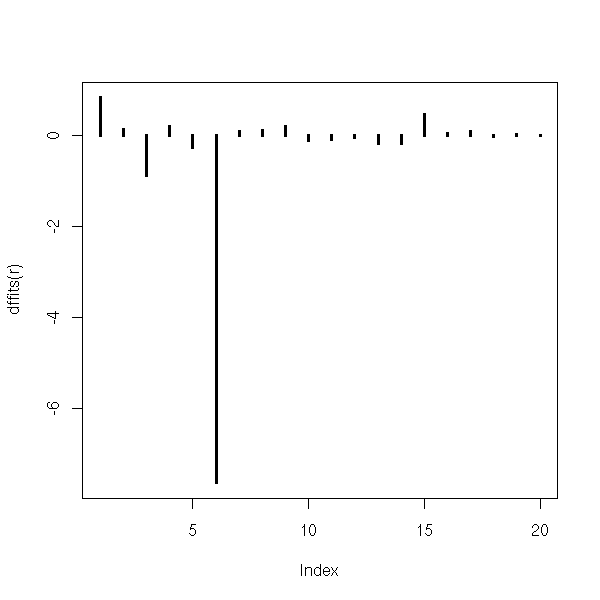
You can also measure the effect of each observation on the regression: remove the point, compute the regression, the predicted values and compare them with the values predicted from the whole sample:
plot(dffits(r),type='h',lwd=3)
You can also compare the coefficients:
plot(dfbetas(r)[,1],type='h',lwd=3)

plot(dfbetas(r)[,2],type='h',lwd=3)

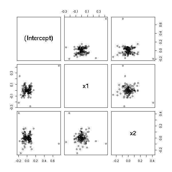
In higher dimensions, you can plot the variation of a coefficient as a function of the variation of other coefficients.
n <- 200
x1 <- rnorm(n)
x2 <- rnorm(n)
yy <- x1 - x2 + rnorm(n)
yy[1] <- 10
r <- lm(yy~x1+x2)
pairs(dfbetas(r))
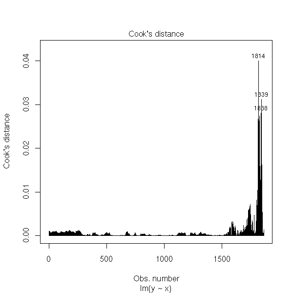
Cook's distance measures the effect of an observation on the regression as a whole. You should start to be cautious when D > 4/n.
cd <- cooks.distance(r)
plot(cd,type='h',lwd=3)

You can also have a look at the box-and-whiskers plot, the scatterplot, the histogram, the density of Cook's distances (for a moment, we put aside our pathological example).
n <- 100
xx <- rnorm(n)
yy <- 1 - 2 * x + rnorm(n)
rr <- lm(yy~xx)
cd <- cooks.distance(rr)
plot(cd,type='h',lwd=3)

boxplot(cd, horizontal=T)
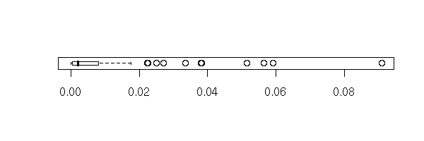
stripchart(cd, method='jitter')

hist(cd, probability=T, breaks=20, col='light blue')

plot(density(cd), type='l', col='red', lwd=3)

qqnorm(cd)
qqline(cd, col='red')

Some suggest to compare the distribution of Cook's distance with a half-gaussian distribution. People often do that for variables whose values are all positive -- but it does not look like a half-gaussian!
half.qqnorm <- function (x) {
  n <- length(x)
  qqplot(qnorm((1+ppoints(n))/2), x)
}
half.qqnorm(cd)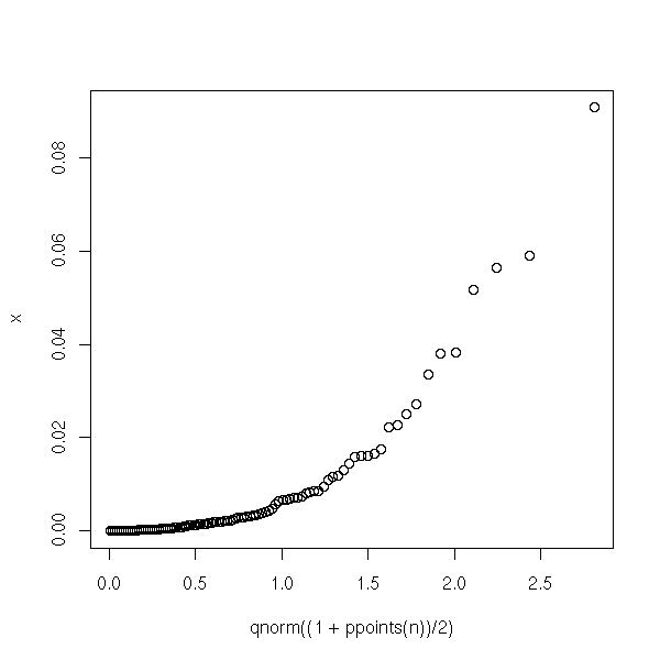
You can use those values to spot the most important points on the scatterplot pr on a residual plot.
m <- max(cooks.distance(r))
plot(y~x, cex=1+5*cooks.distance(r)/m)

cd <- cooks.distance(r)
# rescaled Cook's distance
rcd <- (99/4) * cd*(cd+1)^2
rcd[rcd>100] <- 100
plot(r$res~r$fitted.values, cex=1+.05*rcd)
abline(h=0,lty=3)

You can also use colors.
m <- max(cd)
plot(r$res,
     cex=1+5*cd/m,
     col=heat.colors(100)[ceiling(70*cd/m)],
     pch=16,
    )
points(r$res, cex=1+5*cd/m)
abline(h=0,lty=3)
plot(r$res,
     cex=1+.05*rcd,
     col=heat.colors(100)[ceiling(rcd)],
     pch=16,
    )
points(r$res, cex=1+.05*rcd)
abline(h=0,lty=3)
The following example should be more colorful.
n <- 100
x <- rnorm(n)
y <- 1 - 2*x + rnorm(n)
r <- lm(y~x)
cd <- cooks.distance(r)
m <- max(cd)
plot(r$res ~ r$fitted.values,
     cex=1+5*cd/m,
     col=heat.colors(100)[ceiling(70*cd/m)],
     pch=16,
    )
points(r$res ~ r$fitted.values, cex=1+5*cd/m)
abline(h=0,lty=3)
It might be prettier on a black background.
op <- par(fg='white', bg='black',
          col='white', col.axis='white',
          col.lab='white', col.main='white',
          col.sub='white')
plot(r$res ~ r$fitted.values,
     cex=1+5*cd/m,
     col=heat.colors(100)[ceiling(100*cd/m)],
     pch=16,
    )
abline(h=0,lty=3)
par(op)
You can also have a look at the "lm.influence", "influence.measures", "ls.diag" functions.
TODO: delete the following plot?
# With Cook's distance
x <- rnorm(20)
y <- 1 + x + rnorm(20)
x <- c(x,10)
y <- c(y,1)
r <- lm(y~x)
d <- cooks.distance(r)
d <- (99/4)*d*(d+1)^2 + 1
d[d>100] <- 100
d[d<20] <- 20
d <- d/20
plot( y~x, cex=d )
abline(r)
abline(coef(line(x,y)), col='red')
abline(lm(y[1:20]~x[1:20]),col='blue')
When there is not a single extreme value but several, it is trickier to spot. You can try with a resistant regression, such as a trimmed regression (lts).
Usually, those multiple extreme values do not appear at random (as would an isolated outlier), but have a real meaning -- as such, they should be dealt with. You can try to spot them with unsupervised learning algorithms.
?hclust
?kmeans

TODO: give an example
A cluster of extreme values can also be a sign that the model is not appropriate.
TODO: write up (and model) the following example (mixture)

n <- 200
s <- .2
x <- runif(n)
y1 <- 1 - 2 * x + s*rnorm(n)
y2 <- 2 * x - 1 + s*rnorm(n)
y <- ifelse( sample(c(T,F),n,replace=T,prob=c(.25,.75)), y1, y2 )
plot(y~x)
abline(1,-2,lty=3)
abline(-1,2,lty=3)
If the residuals are not gaussian, the least squares estimators are not optimal (some robust estimators are better, even if they are biased) and, even worse, all the tests, variance computations, confidence interval computations are wrong.
However, if the residuals are less dispersed that with a gaussian distribution or, to a lesser extent, if the sample is very large, you can forget those problems.
You can spot non-gaussian residuals with histograms, box-and-whiskers plots (boxplots) or quantile-quantile plots.
x <- runif(100)
y <- 1 - 2*x + .3*exp(rnorm(100)-1)
r <- lm(y~x)
boxplot(r$residuals, horizontal=T)

hist(r$residuals, breaks=20, probability=T, col='light blue')
lines(density(r$residuals), col='red', lwd=3)
f <- function(x) {
  dnorm(x,
        mean=mean(r$residuals),
        sd=sd(r$residuals),
  )
}
curve(f, add=T, col="red", lwd=3, lty=2)
Do not forget the quantile-quantile plots.
qqnorm(r$residuals)
qqline(r$residuals, col='red')
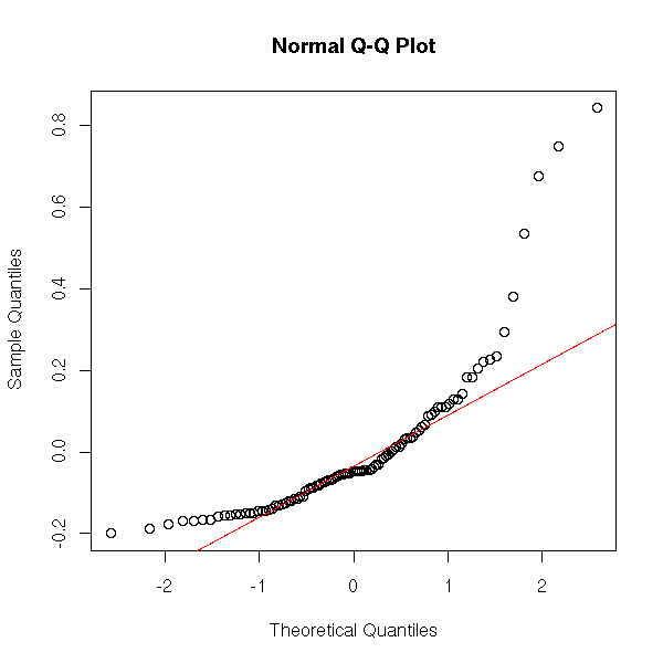
Let us look at what happens with non-gaussian residuals. We shall consider a rather extreme situation: a Cauchy variable with a hole in the middle and a rather small sample.
rcauchy.with.hole <- function (n) {
  x <- rcauchy(n)
  x[x>0] <- 10+x[x>0]
  x[x<0] <- -10+x[x<0]
  x
}
n <- 20
x <- rcauchy(n)
y <- 1 - 2*x + .5*rcauchy.with.hole(n)
plot(y~x)
abline(1,-2)
r <- lm(y~x)
abline(r, col='red')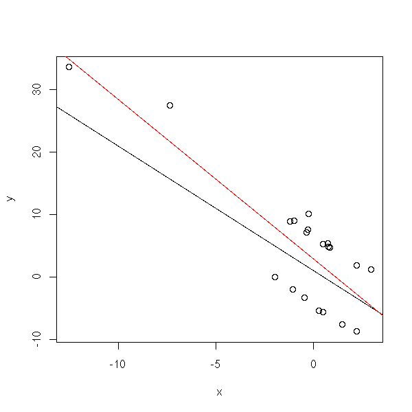
op <- par(mfrow=c(2,2))
hist(r$residuals, breaks=20, probability=T, col='light blue')
lines(density(r$residuals), col='red', lwd=3)
f <- function(x) {
  dnorm(x,
        mean=mean(r$residuals),
        sd=sd(r$residuals),
  )
}
curve(f, add=T, col="red", lwd=3, lty=2)
qqnorm(r$residuals)
qqline(r$residuals, col='red')
plot(r$residuals ~ r$fitted.values)
plot(r$residuals ~ x)
par(op)
Let us compute some forecasts.
n <- 10000
xp <- runif(n,-50,50)
yp <- predict(r, data.frame(x=xp), interval="prediction")
yr <- 1 - 2*xp + .5*rcauchy.with.hole(n)
sum( yr < yp[,3] & yr > yp[,2] )/n
We get 0.9546, i.e., we are in the prediction interval in (more than) 5% of the cases -- but the prediction interval is huge: it tells us that we cannot predict much.
Let us try with a smaller sample.
n <- 5
x <- rcauchy(n)
y <- 1 - 2*x + .5*rcauchy.with.hole(n)
r <- lm(y~x)
n <- 10000
xp <- sort(runif(n,-50,50))
yp <- predict(r, data.frame(x=xp), interval="prediction")
yr <- 1 - 2*xp + .5*rcauchy.with.hole(n)
sum( yr < yp[,3] & yr > yp[,2] )/n
Even worse: 0.9975.
To see what happens, let us plot some of these points.
done <- F
while(!done) {
  # A situation where the prediction interval is not too
  # large, so that it appears on the plot.
  n <- 5
  x <- rcauchy(n)
  y <- 1 - 2*x + .5*rcauchy.with.hole(n)
  r <- lm(y~x)
  n <- 100000
  xp <- sort(runif(n,-50,50))
  yp <- predict(r, data.frame(x=xp), interval="prediction")
  done <- ( yp[round(n/2),2] > -75 & yp[round(n/2),3] < 75 )
}
yr <- 1 - 2*xp + .5*rcauchy.with.hole(n)
plot(yp[,1]~xp, type='l',
     xlim=c(-50,50), ylim=c(-100,100))
points(yr~xp, pch='.')
lines(xp, yp[,2], col='blue')
lines(xp, yp[,3], col='blue')
abline(r, col='red')
points(y~x, col='orange', pch=16, cex=1.5)
points(y~x, cex=1.5)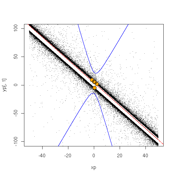
done <- F
while(!done) {
  # Even worse: the sign of the slope is incorrect
  n <- 5
  x <- rcauchy(n)
  y <- 1 - 2*x + .5*rcauchy.with.hole(n)
  r <- lm(y~x)
  n <- 100000
  xp <- sort(runif(n,-50,50))
  yp <- predict(r, data.frame(x=xp), interval="prediction")
  print(r$coef[2])
  done <- ( yp[round(n/2),2] > -75 &
            yp[round(n/2),3] <  75 &
            r$coef[2]>0 )
}
yr <- 1 - 2*xp + .5*rcauchy.with.hole(n)
plot(yp[,1]~xp, type='l',
     xlim=c(-50,50), ylim=c(-100,100))
points(yr~xp, pch='.')
lines(xp, yp[,2], col='blue')
lines(xp, yp[,3], col='blue')
abline(r, col='red')
points(y~x, col='orange', pch=16, cex=1.5)
points(y~x, cex=1.5)
We see that the prediction interval is huge if there are several outliers. Let us try with smaller values.
n <- 10000
xp <- sort(runif(n,-.1,.1))
yp <- predict(r, data.frame(x=xp), interval="prediction")
yr <- 1 - 2*xp + .5*rcauchy.with.hole(n)
sum( yr < yp[,3] & yr > yp[,2] )/n
We get 0.9932...
done <- F
while (!done) {
  n <- 5
  x <- rcauchy(n)
  y <- 1 - 2*x + .5*rcauchy.with.hole(n)
  r <- lm(y~x)
  done <- T
}
n <- 10000
xp <- sort(runif(n,-2,2))
yp <- predict(r, data.frame(x=xp), interval="prediction")
yr <- 1 - 2*xp + .5*rcauchy.with.hole(n)
plot(c(xp,x), c(yp[,1],y), pch='.',
     xlim=c(-2,2), ylim=c(-50,50) )
lines(yp[,1]~xp)
abline(r, col='red')
lines(xp, yp[,2], col='blue')
lines(xp, yp[,3], col='blue')
points(yr~xp, pch='.')
points(y~x, col='orange', pch=16)
points(y~x)
done <- F
essais <- 0
while (!done) {
  n <- 5
  x <- rcauchy(n)
  y <- 1 - 2*x + .5*rcauchy.with.hole(n)
  r <- lm(y~x)
  yp <- predict(r, data.frame(x=2), interval='prediction')
  done <- yp[3]<0
  essais <- essais+1
}
print(essais) # Around 20 or 30
n <- 10000
xp <- sort(runif(n,-2,2))
yp <- predict(r, data.frame(x=xp), interval="prediction")
yr <- 1 - 2*xp + .5*rcauchy.with.hole(n)
plot(c(xp,x), c(yp[,1],y), pch='.',
     xlim=c(-2,2), ylim=c(-50,50) )
lines(yp[,1]~xp)
points(yr~xp, pch='.')
abline(r, col='red')
lines(xp, yp[,2], col='blue')
lines(xp, yp[,3], col='blue')
points(y~x, col='orange', pch=16)
points(y~x)
done <- F
e <- NULL
for (i in 1:100) {
  essais <- 0
  done <- F
  while (!done) {
    n <- 5
    x <- rcauchy(n)
    y <- 1 - 2*x + .5*rcauchy.with.hole(n)
    r <- lm(y~x)
    yp <- predict(r, data.frame(x=2), interval='prediction')
    done <- yp[3]<0
    essais <- essais+1
  }
  e <- append(e,essais)
}
hist(e, probability=T, col='light blue')
lines(density(e), col='red', lwd=3)
abline(v=median(e), lty=2, col='red', lwd=3)
> mean(e)
[1] 25.8
> median(e)
[1] 19
In short, to have the most incorrect prediction intervals, take large values of x, bit not too large (close to 0, the predictions are correct, away from 0, the prediction intervals are huge).
I wanted to prove, here, on an example, that non gaussian residuals produces confidence intervals too small and thus incorrect results. I was wrong: the confidence intervals are correct but very large, to the point that the forecasts are useless.
Exercice: do the same with other distributions (Cauchy, uniform, etc.), either for the noise or for the variables.
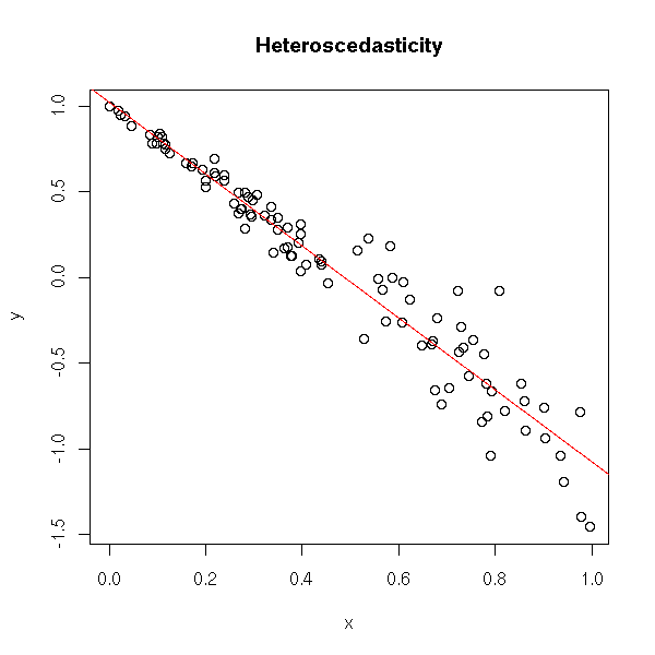
For the least squares estimators to be optimal and for the test results to be correct, we had to assume (among other hypotheses) that the variance of the noise was constant. If it is not, it is said toe be heteroscedastic.
x <- runif(100)
y <- 1 - 2*x + .3*x*rnorm(100)
plot(y~x)
r <- lm(y~x)
abline(r, col='red')
title(main="Heteroscedasticity")
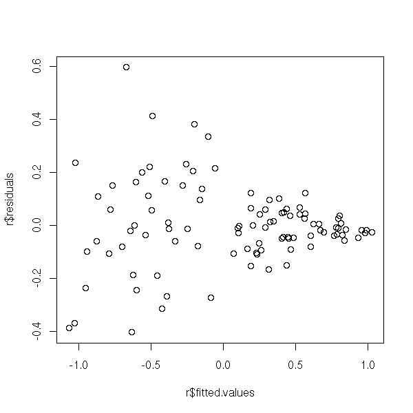
You can spot the problem on the residuals.
plot(r$residuals ~ r$fitted.values)
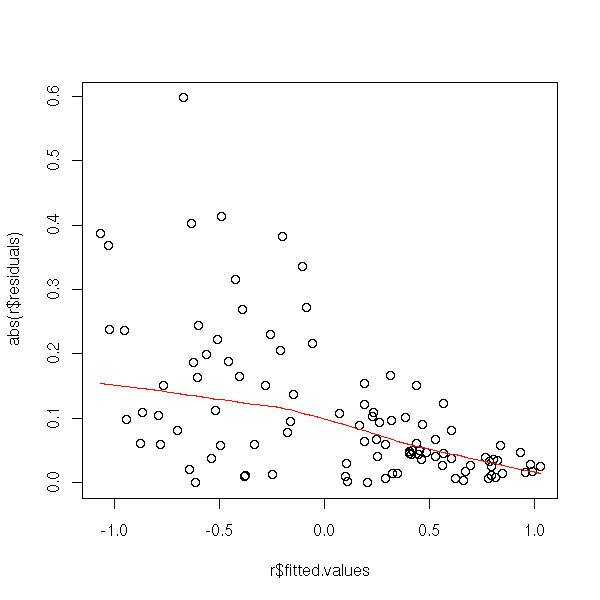
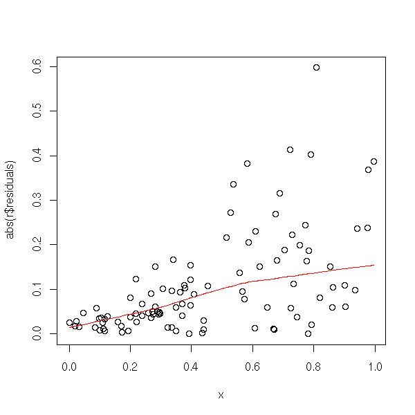
Or, more precisely, on their absolute value, on which you can perform a non-linear regression.
plot(abs(r$residuals) ~ r$fitted.values)
lines(lowess(r$fitted.values, abs(r$residuals)), col='red')
plot(abs(r$residuals) ~ x)
lines(lowess(x, abs(r$residuals)), col='red')
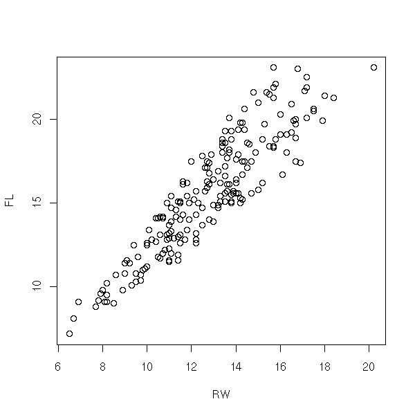
Here is a concrete example.
data(crabs)
plot(FL~RW, data=crabs)
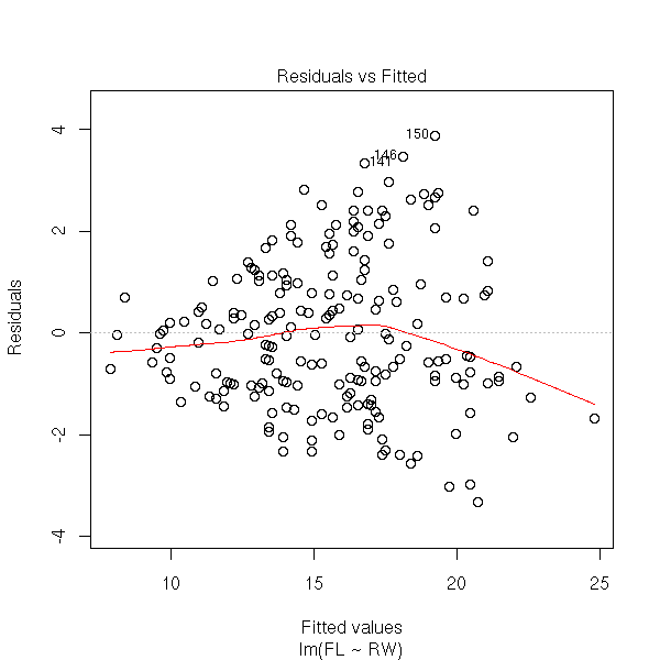
r <- lm(FL~RW, data=crabs)
plot(r, which=1)
plot(r, which=3, panel = panel.smooth)

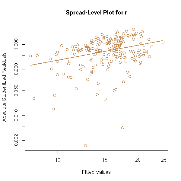
The "spread.level.plot" from the "car" package has the same aim: it plots the absolute value of the residuals as a function of the predicted values, on logarithmic scales and suggests a transformation to get rid of heteroscedasticity.
library(car)
spread.level.plot(r)
You can also see the problem in a more computational way, by splitting the sample into two parts and performing a test to see if the two parts have the same variance.
n <- length(crabs$RW)
m <- ceiling(n/2)
o <- order(crabs$RW)
r <- lm(FL~RW, data=crabs)
x <- r$residuals[o[1:m]]
y <- r$residuals[o[(m+1):n]]
var.test(y,x) # p-value = 1e-4
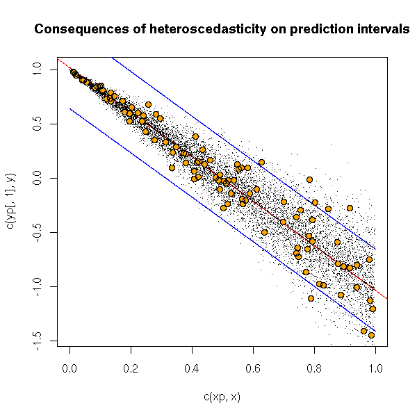
Let us see, on an example, what the effects of heteroscedasticity are.
x <- runif(100)
y <- 1 - 2*x + .3*x*rnorm(100)
r <- lm(y~x)
xp <- runif(10000,0,.1)
yp <- predict(r, data.frame(x=xp), interval="prediction")
yr <- 1 - 2*xp + .3*xp*rnorm(100)
sum( yr < yp[,3] & yr > yp[,2] )/n
We get 1: where the variance is small, the confidence intervals are too small.
x <- runif(100)
y <- 1 - 2*x + .3*x*rnorm(100)
r <- lm(y~x)
xp <- runif(10000,.9,1)
yp <- predict(r, data.frame(x=xp), interval="prediction")
yr <- 1 - 2*xp + .3*xp*rnorm(100)
sum( yr < yp[,3] & yr > yp[,2] )/n
We get 0.67: where the variance is higher, the confidence intervals are too small.
We can see this graphically.
x <- runif(100)
y <- 1 - 2*x + .3*x*rnorm(100)
r <- lm(y~x)
n <- 10000
xp <- sort(runif(n,))
yp <- predict(r, data.frame(x=xp), interval="prediction")
yr <- 1 - 2*xp + .3*xp*rnorm(n)

plot(c(xp,x), c(yp[,1],y), pch='.')
lines(yp[,1]~xp)
abline(r, col='red')
lines(xp, yp[,2], col='blue')
lines(xp, yp[,3], col='blue')
points(yr~xp, pch='.')
points(y~x, col='orange', pch=16)
points(y~x)
title(main="Consequences of heteroscedasticity on prediction intervals")
The simplest way to get rid of heteroscedasticity is (when it works) to transform the data. If it is possible, find a transformation of the data that will both have it look gaussian and get rid of heteroscedasticity.
Generalized least squaes allow you to perform a regression with heteroscedastic data, but you have to know how the variance varies.
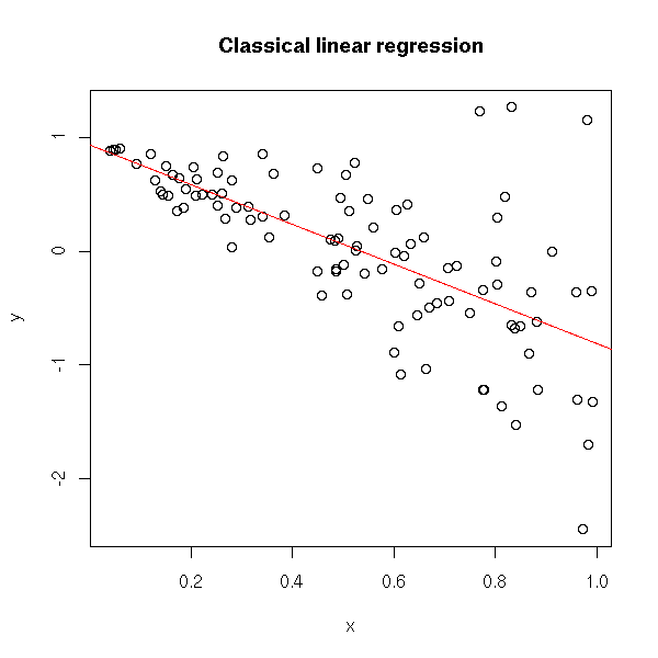
TODO: put this example later?

n <- 100
x <- runif(n)
y <- 1 - 2*x + x*rnorm(n)
plot(y~x)
r <- lm(y~x)
abline(r, col='red')
title(main="Classical linear regression")
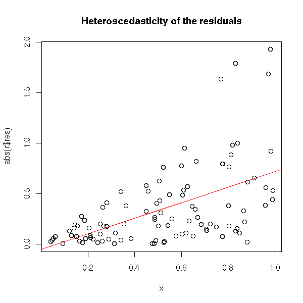
plot(abs(r$res) ~ x)
r2 <- lm( abs(r$res) ~ x )
abline(r2, col="red")
title(main="Heteroscedasticity of the residuals")
The idea of weighted least squares is to give a lesser weight (i.e., a lesser importance) to observations whose variance is high.
# We assume the the standard deviation of the residuals
# is of the form a*x
a <- lm( I(r$res^2) ~ I(x^2) - 1 )$coefficients
w <- (a*x)^-2
r3 <- lm( y ~ x, weights=w )
plot(y~x)
abline(1,-2, lty=3)
abline(lm(y~x), lty=3, lwd=3)
abline(lm(y~x, weights=w), col='red')
legend( par("usr")[1], par("usr")[3], yjust=0,
        c("acutal model", "least squares",
          "weighted least squares"),
        lwd=c(1,3,1),
        lty=c(3,3,1),
        col=c(par("fg"), par("fg"), 'red') )
title("Weighted least squares and heteroscedasticity")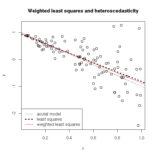
On the contrary, the prediction intervals are not very convincing...
TODO: check what follows

# Prediction intervals
N <- 10000
xx <- runif(N,min=0,max=2)
yy <- 1 - 2*xx + xx*rnorm(N)
plot(y~x, xlim=c(0,2), ylim=c(-3,2))
points(yy~xx, pch='.')
abline(1,-2, col='red')
xp <- seq(0,3,length=100)
yp1 <- predict(r, new=data.frame(x=xp), interval='prediction')
lines( xp, yp1[,2], col='red', lwd=3 )
lines( xp, yp1[,3], col='red', lwd=3 )
yp3 <- predict(r3, new=data.frame(x=xp), interval='prediction')
lines( xp, yp3[,2], col='blue', lwd=3 )
lines( xp, yp3[,3], col='blue', lwd=3 )
legend( par("usr")[1], par("usr")[3], yjust=0,
        c("least squares", "weighted least squares"),
        lwd=3, lty=1,
        col=c('red', 'blue') )
title(main="Prediction band")
You can also do that with the "gls" function
?gls
?varConstPower
?varPower

r4 <- gls(y~x, weights=varPower(1, form= ~x))
???
library(help=lmtest)
library(help=strucchange)

# Heteroscedasticity
library(lmtest)
?dwtest
?bgtest
?bptest
?gqtest
?hmctest
In the case of time series, of geographical data (or more generally, data for which you ave a notion of "proximity" between the observations), the errors of two consecutive observations may be correlated.
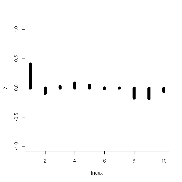
In the case of time series, you can see the problem in an autocorrelogram.
my.acf.plot <- function (x, n=10, ...) {
  y <- rep(NA,n)
  l <- length(x)
  for (i in 1:n) {
    y[i] <- cor( x[1:(l-i)], x[(i+1):l] )
  }
  plot(y, type='h', ylim=c(-1,1),...)
}
n <- 100
x <- runif(n)
b <- .1*rnorm(n+1)
y <- 1-2*x+b[1:n]
my.acf.plot(lm(y~x)$res, lwd=10)
abline(h=0, lty=2)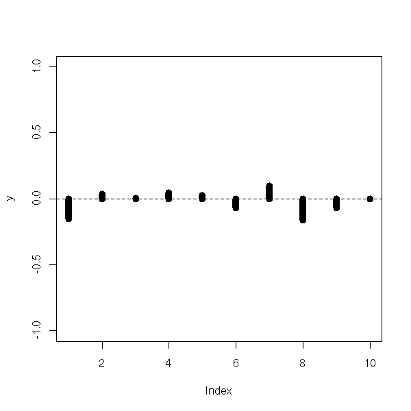
z <- 1-2*x+.5*(b[1:n]+b[1+1:n])
my.acf.plot(lm(z~x)$res, lwd=10)
abline(h=0, lty=2)
Here is a very autocorrelated example.
n <- 500
x <- runif(n)
b <- rep(NA,n)
b[1] <- 0
for (i in 2:n) {
  b[i] <- b[i-1] + .1*rnorm(1)
}
y <- 1-2*x+b[1:n]
my.acf.plot(lm(y~x)$res, n=100)
abline(h=0, lty=2)
title(main='Very autocorrelated example')
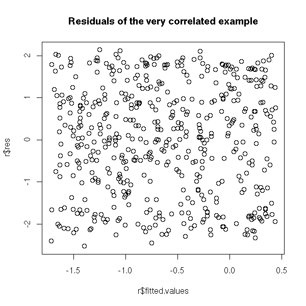
We do not see anything on the plot of the residuals as a function of the predicted values.
r <- lm(y~x)
plot(r$res ~ r$fitted.values)
title(main="Residuals of the very correlated example")
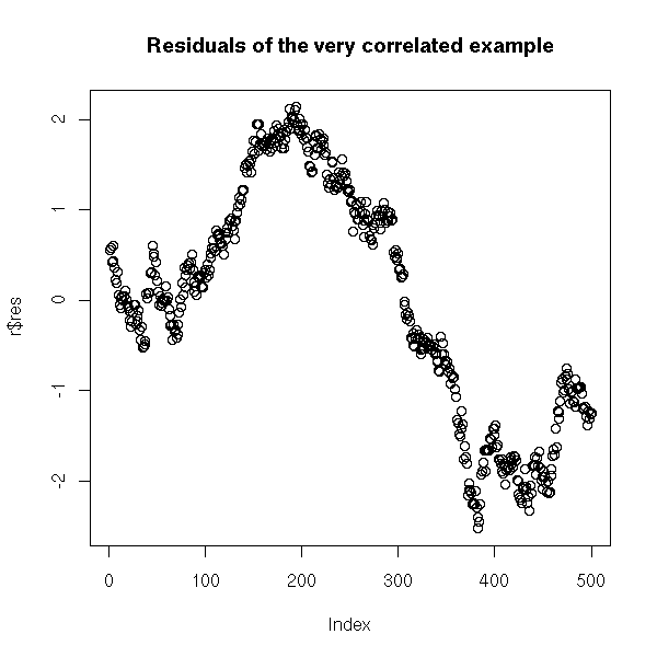
On the contrary, if you plot the residuals as a function of time, it is clearer.
r <- lm(y~x)
plot(r$res)
title(main="Residuals of the very correlated example")
Another means of spotting the problem is to check if the correlation between x[i] and x[i-1] is significantly non zero.
n <- 100
x <- runif(n)
b <- rep(NA,n)
b[1] <- 0
for (i in 2:n) {
  b[i] <- b[i-1] + .1*rnorm(1)
}
y <- 1-2*x+b[1:n]
r <- lm(y~x)$res
cor.test(r[1:(n-1)], r[2:n]) # p-value under 1e-15

n <- 100
x <- runif(n)
b <- .1*rnorm(n+1)
y <- 1-2*x+b[1:n]
r <- lm(y~x)$res
cor.test(r[1:(n-1)], r[2:n]) # p-value = 0.3

y <- 1-2*x+.5*(b[1:n]+b[1+1:n])
cor.test(r[1:(n-1)], r[2:n]) # p-value = 0.3 (again)
See also the Durbin--Watson test:
library(car)
?durbin.watson

library(lmtest)
?dwtest
and the chapter on time series.
Yet another means of spotting the problem is to plot the consecutive residuals in 2 or 3 dimensions.
n <- 500
x <- runif(n)
b <- rep(NA,n)
b[1] <- 0
for (i in 2:n) {
  b[i] <- b[i-1] + .1*rnorm(1)
}
y <- 1-2*x+b[1:n]
r <- lm(y~x)$res
plot( r[1:(n-1)], r[2:n],
      xlab='i-th residual',
      ylab='(i+1)-th residual' )
In the following example, we do not see anything with two consecutive terms (well, it looks like a Rorschach test, it is suspicious): we need three.
n <- 500
x <- runif(n)
b <- rep(NA,n)
b[1] <- 0
b[2] <- 0
for (i in 3:n) {
  b[i] <- b[i-2] + .1*rnorm(1)
}
y <- 1-2*x+b[1:n]
r <- lm(y~x)$res
plot(data.frame(x=r[3:n-2], y=r[3:n-1], z=r[3:n]))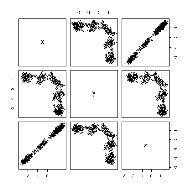
plot(r)

It is exaclty like that we can see the problems of some old random number generators. In three dimensions, front view, there is nothing visible,
data(randu)
plot(randu)
# Nothing visible
but if we rotate the figure...
library(xgobi)
xgobi(randu)

You can also turn the picture directly in R, by taking a "random" rotation matrix (exercice: write a function to produce such a matrix -- hint: there is one somewhere inthis document).
m <- matrix( c(0.0491788982891203, -0.998585856299176, 0.0201921658647648,
               0.983046639705112,  0.0448184901961194, -0.177793720645666,
               -0.176637312387723,  -0.028593540105802, -0.983860594462783),
             nr=3, nc=3)
plot( t( m %*% t(randu) )[,1:2] )
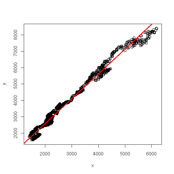
Here is a real example.
data(EuStockMarkets)
plot(EuStockMarkets)

x <- EuStockMarkets[,1]
y <- EuStockMarkets[,2]
r <- lm(y~x)
plot(y~x)
abline(r, col='red', lwd=3)
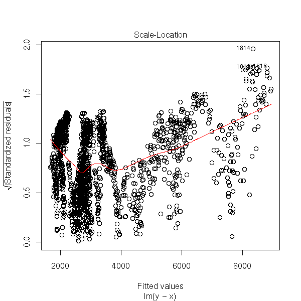
plot(r, which=1)

plot(r, which=3)
plot(r, which=4)
r <- r$res
hist(r, probability=T, col='light blue')
lines(density(r), col='red', lwd=3)

plot(r)

acf(r)

pacf(r)

r <- as.vector(r)
x <- r[1:(length(r)-1)]
y <- r[2:length(r)]
plot(x,y, xlab='x[i]', ylab='x[i+1]')

In such a situation, you can use generalized least squares. The AR1 model assumes that two successive errors are correlated:
e_{i+1} = r * e_i + f_iWhere r is the "AR1 coefficient" and the f_i are independant.
n <- 100
x <- rnorm(n)
e <- vector()
e <- append(e, rnorm(1))
for (i in 2:n) {
  e <- append(e, .6 * e[i-1] + rnorm(1) )
}
y <- 1 - 2*x + e
i <- 1:n
plot(y~x)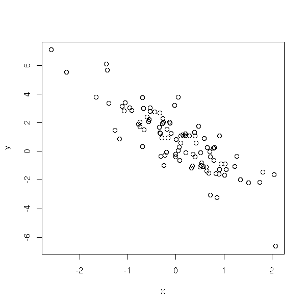
r <- lm(y~x)$residuals
plot(r)

The "gls" function (generalized least squares) is in the "nlme" package.
library(nlme)
g <- gls(y~x, correlation = corAR1(form= ~i))
Here is the result.
> summary(g)
Generalized least squares fit by REML
  Model: y ~ x
  Data: NULL
       AIC      BIC    logLik
  298.4369 308.7767 -145.2184

Correlation Structure: AR(1)
 Formula: ~i
 Parameter estimate(s):
      Phi
0.3459834

Coefficients:
                Value  Std.Error    t-value p-value
(Intercept)  1.234593 0.15510022   7.959971  <.0001
x           -1.892171 0.09440561 -20.042992  <.0001

 Correlation:
  (Intr)
x 0.04

Standardized residuals:
        Min          Q1         Med          Q3         Max
-2.14818684 -0.75053384  0.02200128  0.57222518  2.45362824

Residual standard error: 1.085987
Degrees of freedom: 100 total; 98 residual
We can look at the confidence interval on the autocorrelation coefficient.
> intervals(g)
Approximate 95% confidence intervals

 Coefficients:
                lower      est.     upper
(Intercept)  0.926802  1.234593  1.542385
x           -2.079516 -1.892171 -1.704826

 Correlation structure:
        lower      est.     upper
Phi 0.1477999 0.3459834 0.5174543

 Residual standard error:
   lower     est.    upper
0.926446 1.085987 1.273003
Let us compare with a naive regression.
library(nlme)
plot(y~x)
abline(lm(y~x))
abline(gls(y~x, correlation = corAR1(form= ~i)), col='red')
In this example, there is no remarkable effect. In the following, the situation is more drastic.
n <- 1000
x <- rnorm(n)
e <- vector()
e <- append(e, rnorm(1))
for (i in 2:n) {
  e <- append(e, 1 * e[i-1] + rnorm(1) )
}
y <- 1 - 2*x + e
i <- 1:n
plot(lm(y~x)$residuals)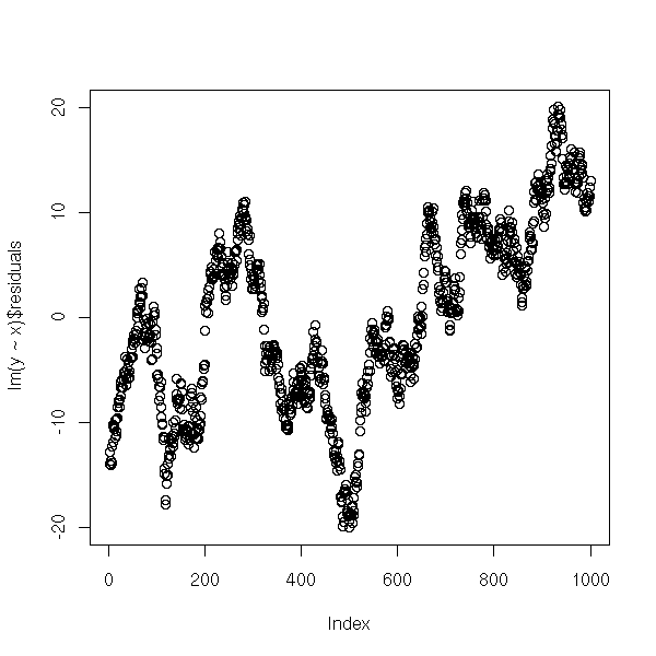
plot(y~x)
abline(lm(y~x))
abline(gls(y~x, correlation = corAR1(form= ~i)), col='red')
abline(1,-2, lty=2)
We shall come back on this when we tackle time series.
For spatial data, it is more complicated.
TODO: a reference???
The correlation coefficient between two variables tells you if they are correlated. But you can also have relations between more than two variables, such as X3 = X1 + X2. To detect those, you can perform a regression of Xk agains the other Xi's and check the R^2: if it is high (>1e-1), Xk can be expressed from the other Xi.
n <- 100
x <- rnorm(n)
x1 <- x+rnorm(n)
x2 <- x+rnorm(n)
x3 <- rnorm(n)
y <- x+x3
summary(lm(x1~x2+x3))$r.squared  # 1e-1
summary(lm(x2~x1+x3))$r.squared  # 1e-1
summary(lm(x3~x1+x2))$r.squared  # 1e-3
Other example, with three dependant variables.
n <- 100
x1 <- rnorm(n)
x2 <- rnorm(n)
x3 <- x1+x2+rnorm(n)
x4 <- rnorm(n)
y <- x1+x2+x3+x4+rnorm(n)
summary(lm(x1~x2+x3+x4))$r.squared  # 0.5
summary(lm(x2~x1+x3+x4))$r.squared  # 0.4
summary(lm(x3~x1+x2+x4))$r.squared  # 0.7
summary(lm(x4~x1+x2+x3))$r.squared  # 3e-3
Real example (with the adjusted determination coefficient):
check.multicolinearity <- function (M) {
  a <- NULL
  n <- dim(M)[2]
  for (i in 1:n) {
    m <- as.matrix(M[, 1:n!=i])
    y <- M[,i]
    a <- append(a, summary(lm(y~m))$adj.r.squared)
  }
  names(a) <- names(M)
  print(round(a,digits=2))
  invisible(a)
}
data(freeny)
names(freeny) <- paste(
  names(freeny),
  " (",
  round(check.multicolinearity(freeny), digits=2),
  ")",
  sep='')
pairs(freeny,
  upper.panel=panel.smooth,
  lower.panel=panel.smooth)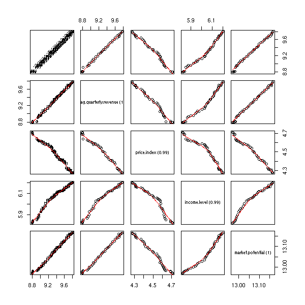
In such a situation, the fact that a certain coefficient be statistically different from zero depends on the presence of other variables. With all the variables, the first variables does not play a significant role, but the second does.
> summary(lm(freeny.y ~ freeny.x))
...
Coefficients:
                              Estimate Std. Error t value Pr(>|t|)
(Intercept)                   -10.4726     6.0217  -1.739   0.0911 .
freeny.xlag quarterly revenue   0.1239     0.1424   0.870   0.3904
freeny.xprice index            -0.7542     0.1607  -4.693 4.28e-05 ***
freeny.xincome level            0.7675     0.1339   5.730 1.93e-06 ***
freeny.xmarket potential        1.3306     0.5093   2.613   0.0133 *
...
Multiple R-Squared: 0.9981,     Adjusted R-squared: 0.9978
On the contrary, if you only retain the first two variables, it is the opposite.
> summary(lm(freeny.y ~ freeny.x[,1:2]))
...
                                     Estimate Std. Error t value Pr(>|t|)
(Intercept)                           2.18577    1.47236   1.485    0.146
freeny.x[, 1:2]lag quarterly revenue  0.89122    0.07412  12.024 3.63e-14 ***
freeny.x[, 1:2]price index           -0.25592    0.17534  -1.460    0.153
...
Multiple R-Squared: 0.9958,     Adjusted R-squared: 0.9956
Furthermore, the estimation of the coefficients anf their standard deviation is worrying: in a multilinearity situation, you cannot be sure of the sign of the coefficients.
n <- 100
v <- .1
x <- rnorm(n)
x1 <- x + v*rnorm(n)
x2 <- x + v*rnorm(n)
x3 <- x + v*rnorm(n)
y <- x1+x2-x3 + rnorm(n)
Let us check that the variables are linearly dependant.
> summary(lm(x1~x2+x3))$r.squared
[1] 0.986512
> summary(lm(x2~x1+x3))$r.squared
[1] 0.98811
> summary(lm(x3~x1+x2))$r.squared
[1] 0.9862133
Let us look at the most relevant ones.
> summary(lm(y~x1+x2+x3))

Call:
lm(formula = y ~ x1 + x2 + x3)

Residuals:
    Min      1Q  Median      3Q     Max
-3.0902 -0.7658  0.0793  0.6995  2.6456

Coefficients:
            Estimate Std. Error t value Pr(>|t|)
(Intercept)  0.06361    0.11368   0.560   0.5771
x1           1.47317    0.94653   1.556   0.1229
x2           1.18874    0.98481   1.207   0.2304
x3          -1.70372    0.94366  -1.805   0.0741 .
---
Signif. codes:  0 `***' 0.001 `**' 0.01 `*' 0.05 `.' 0.1 ` ' 1

Residual standard error: 1.135 on 96 degrees of freedom
Multiple R-Squared: 0.4757,     Adjusted R-squared: 0.4593
F-statistic: 29.03 on 3 and 96 DF,  p-value: 1.912e-13
It is the third.
> lm(y~x3)$coef
(Intercept)          x3
 0.06970513  0.98313878
Its coefficient was negative, but if we remove the other variables, it becomes positive.
Instead of looking at the determination coefficient (percentage of explained variance) R^2, you can look at the "Variance Inflation Factors" (VIF),
          1
V_j = -----------
       1 - R_j^2

> vif(lm(y~x1+x2+x3))
      x1       x2       x3
48.31913 41.13990 52.10746
Instead of looking at the R^2, you can look at the correlation matrix between the estimated coefficients.
n <- 100
v <- .1
x <- rnorm(n)
x1 <- x + v*rnorm(n)
x2 <- rnorm(n)
x3 <- x + v*rnorm(n)
y <- x1+x2-x3 + rnorm(n)
summary(lm(y~x1+x2+x3), correlation=T)$correlation
We get
             (Intercept)          x1            x2          x3
(Intercept)  1.0000000000 -0.02036269  0.0001812560  0.02264558
x1          -0.0203626936  1.00000000 -0.1582002900 -0.98992751
x2           0.0001812560 -0.15820029  1.0000000000  0.14729488
x3           0.0226455841 -0.98992751  0.1472948846  1.00000000
We can see that X1 and X3 are dependant. We can also see it graphically.
n <- 100
v <- .1
x <- rnorm(n)
x1 <- x + v*rnorm(n)
x2 <- rnorm(n)
x3 <- x + v*rnorm(n)
y <- x1+x2-x3 + rnorm(n)
m <- summary(lm(y~x1+x2+x3), correlation=T)$correlation
plot(col(m), row(m), cex=10*abs(m),
     xlim=c(0, dim(m)[2]+1),
     ylim=c(0, dim(m)[1]+1),
     main="Correlation matrix of the coefficients of a regression")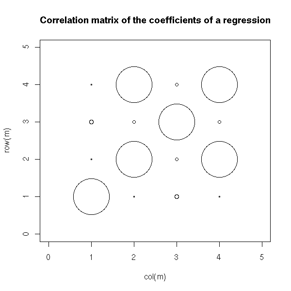
TODO: A graphical representation of this correlation matrix (transform it into a distance matrix, perform an MDS, plot the points, add their MST -- or simply plot the MST, without the MDS).
Here is yet another way of spotting the problem: compute the ratio of the largest eigen value and the smallest. Under 100, it is fine, over 1000, it is worrying. This is called the "contitionning index".
m <- model.matrix(y~x1+x2+x3)
d <- eigen( t(m) %*% m, symmetric=T )$values
d[1]/d[4] # 230
To solve the problem, you can remove the "superfluous" variables -- but you might run into interpretation problems. You can also ask for more data (multicolinearity are more frequent when you have many variables and few observations). You can also use regression techniques adapted to multicolinearity, such as "ridge regression" or SVM (see somewhere below).
We have already run into this problem with polynomial regression: to get rid of multicolinearity, we had orthonormalized the predictive variables.
> y <- cars$dist
> x <- cars$speed
> m <- cbind(x, x^2, x^3, x^4, x^5)
> cor(m)
          x
x 1.0000000 0.9794765 0.9389237 0.8943823 0.8515996
  0.9794765 1.0000000 0.9884061 0.9635754 0.9341101
  0.9389237 0.9884061 1.0000000 0.9927622 0.9764132
  0.8943823 0.9635754 0.9927622 1.0000000 0.9951765
  0.8515996 0.9341101 0.9764132 0.9951765 1.0000000

> m <- poly(x,5)
> cor(m)
              1             2             3             4             5
1  1.000000e+00  6.409668e-17 -1.242089e-17 -3.333244e-17  7.935005e-18
2  6.409668e-17  1.000000e+00 -4.468268e-17 -2.024748e-17  2.172470e-17
3 -1.242089e-17 -4.468268e-17  1.000000e+00 -6.583818e-17 -1.897354e-18
4 -3.333244e-17 -2.024748e-17 -6.583818e-17  1.000000e+00 -4.903304e-17
5  7.935005e-18  2.172470e-17 -1.897354e-18 -4.903304e-17  1.000000e+00
TODO: Give the example of mixed models
Adding a subject-dependant intercept is equivalent to imposing a
certain correlation structure.
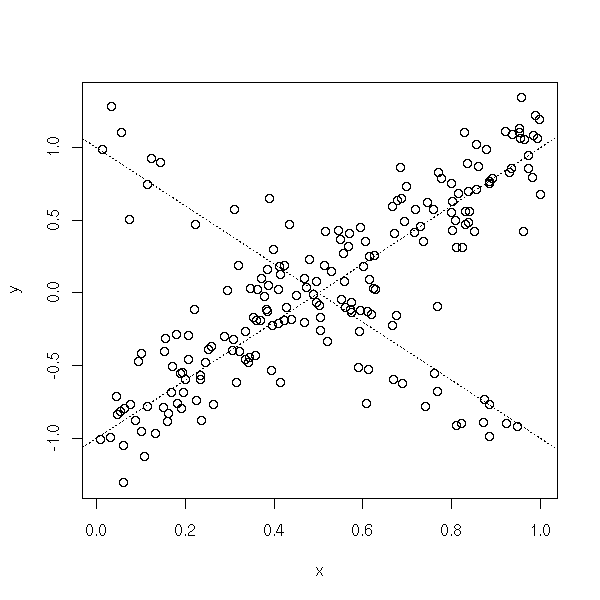
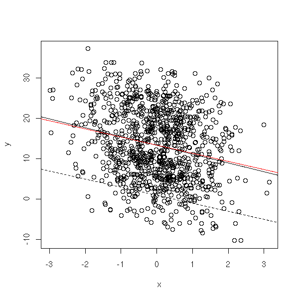
Important variables may be missing, that can change the results of the regression and their interpretation.
In the following example, we have three variables.
n <- 100
x <- runif(n)
z <- ifelse(x>.5,1,0)
y <- 2*z -x + .1*rnorm(n)
plot( y~x, col=c('red','blue')[1+z] )
If we take into account the three variables, there is a negative correlation between x and y.
> summary(lm( y~x+z ))

Call:
lm(formula = y ~ x + z)

Residuals:
      Min        1Q    Median        3Q       Max
-0.271243 -0.065745  0.002929  0.068085  0.215251

Coefficients:
            Estimate Std. Error t value Pr(>|t|)
(Intercept)  0.01876    0.02404    0.78    0.437
x           -1.05823    0.07126  -14.85   <2e-16 ***
z            2.05321    0.03853   53.28   <2e-16 ***
---
Signif. codes:  0 `***' 0.001 `**' 0.01 `*' 0.05 `.' 0.1 ` ' 1

Residual standard error: 0.1008 on 97 degrees of freedom
Multiple R-Squared: 0.9847,     Adjusted R-squared: 0.9844
F-statistic:  3125 on 2 and 97 DF,  p-value: < 2.2e-16
On the contrary, if we do not have z, the correlation becomes positive.
> summary(lm( y~x ))

Call:
lm(formula = y ~ x)

Residuals:
     Min       1Q   Median       3Q      Max
-1.05952 -0.38289 -0.01774  0.50598  1.05198

Coefficients:
            Estimate Std. Error t value Pr(>|t|)
(Intercept)  -0.5689     0.1169  -4.865 4.37e-06 ***
x             2.1774     0.2041  10.669  < 2e-16 ***
---
Signif. codes:  0 `***' 0.001 `**' 0.01 `*' 0.05 `.' 0.1 ` ' 1

Residual standard error: 0.5517 on 98 degrees of freedom
Multiple R-Squared: 0.5374,     Adjusted R-squared: 0.5327
F-statistic: 113.8 on 1 and 98 DF,  p-value: < 2.2e-16
To avoid this problem, you should include all the variables that are likely to be important (you select them from a prior knowledge of the domain studied, i.e., with non-statistical methods).
To confirm a given effect, you can also try other models (if they all confirm the effect, and its direction, it is a good omen) or gather more data, either from the same experiment, or from a comparable but slightly different one.
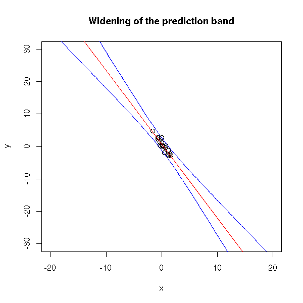
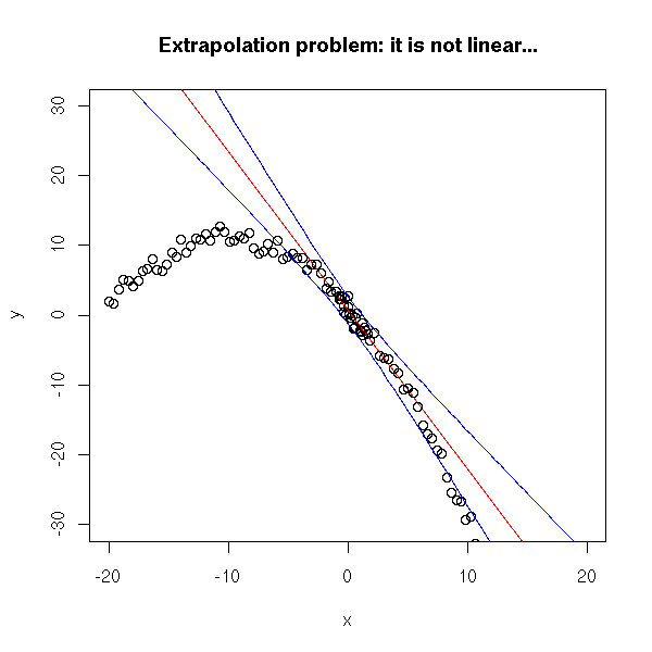
You often want to extrapolate from your data, i.e., infer what happens at larger scale (say, you have data with X in [0,1] and you would like conclusions for X in [0,10]). Several problems occur. The first is that the prediction intervals increase when you get away from the sample values.
n <- 20
x <- rnorm(n)
y <- 1 - 2*x - .1*x^2 + rnorm(n)
#summary(lm(y~poly(x,10)))
plot(y~x, xlim=c(-20,20), ylim=c(-30,30))
r <- lm(y~x)
abline(r, col='red')
xx <- seq(-20,20,length=100)
p <- predict(r, data.frame(x=xx), interval='prediction')
lines(xx,p[,2],col='blue')
lines(xx,p[,3],col='blue')
title(main="Widening of the prediction band")
Furthermore, if the relation looks linear on a small scale, it might be completely different on a larger scale.
plot(y~x, xlim=c(-20,20), ylim=c(-30,30))
r <- lm(y~x)
abline(r, col='red')
xx <- seq(-20,20,length=100)
yy <- 1 - 2*xx - .1*xx^2 + rnorm(n)
p <- predict(r, data.frame(x=xx), interval='prediction')
points(yy~xx)
lines(xx,p[,2],col='blue')
lines(xx,p[,3],col='blue')
title(main="Extrapolation problem: it is not linear...")
data(cars)
y <- cars$dist
x <- cars$speed
o <- x<quantile(x,.25)
x1 <- x[o]
y1 <- y[o]
r <- lm(y1~x1)
xx <- seq(min(x),max(x),length=100)
p <- predict(r, data.frame(x1=xx), interval='prediction')
plot(y~x)
abline(r, col='red')
lines(xx,p[,2],col='blue')
lines(xx,p[,3],col='blue')

If you give the same data to different persons (for instance, students, in an exam), each will have a different model with different forecasts. The forecasts and the corresponding confidence intervals are usually incompatible: the prediction intervals are always too small...
There can be measurement errors on the predictive variable: this yields to biased estimations of the parameters (towards 0).
n <- 100
e <- .5
x0 <- rnorm(n)
x <- x0 + e*rnorm(n)
y <- 1 - 2*x0 + e*rnorm(n)
plot(y~x)
points(y~x0, col='red')
abline(lm(y~x))
abline(lm(y~x0),col='red')
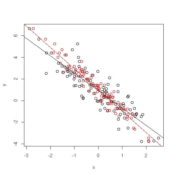
On the other hand, there is no problem about the predictions, because the measurement errors will always be present and are accounted for.
TODO: proofread this. In particular, mention the dangers
of variable selection.
There are actually two different subjects here:
 - the curse of dimension
 - combining models
The curse of dimension
TODO: put this part after the other regressions (logistic, Poisson, ordinal, multilogistic).
TODO: write this part.
TODO: I mainly mention non-linear models in high dimensions. But what can one do when there are more variables than observations? See: svm (support vector machines).
We have already mentionned the "curse of dimension": what can we do when we have more variables than observations? What can we do when we want a non-linear regression with a very large number of variables: In both cases, if we try to play the game as in two dimensions, we end up with too many parameters to estimate with respect to the number of available observations. Either we cannot gat any estimation, or the estimations are almost random (somewhere else in this document, we call this "overfit").
We can turn around the problem by choosing simpler models, models with fewer variables -- simpler, but not too simple: the model has to be sufficiently complex to describe the data.
The following regression methods lie between linear regression (relevant when there are too few observations to allow anything else, or when the data is too noisy) and multiimensional non-linear regression (unuseable, because there are too many parameters to estimate). The allow us to thwart the curse of dimension. More precisely, we shall mention variable selection, principal component regression, ridge regression, lasso, partial least squares, Generalized Additive Models (GAMs) and tree-based algorith,s (CART, MARS).
TODO: give the structure of this chapter
Putative structure of this chapter:
Variables selection
GAM, ACE?, AVAS?
Trees: CART, MARS
Bootstrap: bagging, boosting
  (But there is already a chapter about the bootstrap -- the
  previous chapter...)
Remark: Not all the methods we shall mention seem to be implemented in R.
When facing real data with a very large number of variables, we shall first reduce the dimension, for instance, by selecting the "most relevant" variables and discarding the others.
But how do we do that?
TODO
(This is a good question...)
Here are a few ideas (beware: not all thes ideas are good).
Compute a PCA and "round" the components to the "nearest"
variables.

Reverse the problem and look at the variables: are some of
them "close", in some sense (e.g., define a notion of
distance between the variables and perform a distance
analysis). Then, retain a single variables from each
cluster.
TO SORT

Variables selection to predict a qualitative variables
1. Perform ANOVAs and only retain important variables (say, p-value>0.05)
n <- 100
k <- 5
x <- matrix(rnorm(n*k),nc=k)
y <- x[,1] + x[,2] - sqrt(abs(x[,3]*x[,4]))
y <- y-median(y)
y <- factor(y>0)
pairs(x, col=as.numeric(y)+1)

for (i in 1:k) {
  f <- summary(lm(x[,i]~y))$fstatistic
  f <- pf(f[1],f[2],f[3], lower.tail=F)
  print(paste(i, ";  p =", round(f, digits=3)))
}

2. With the retained variables, compute the correlations and their
   p-values (the p-value of a correlation if the p-value of the test
   of H0: "correlation=0".
TODO: gove an example with colinear variables.
cor(x)
round(cor(x),digits=3)
m <- cor(x)
for (i in 1:k) {
  for (j in 1:k) {
    m[i,j] <- cor.test(x[,i],x[,j])$p.value
  }
}
m
round(m,digits=3)
m<.05

Exercise: write a "print" method for correlation matrices
that adds stars besides the correlations significantly different
from zero.
When there are too many perdictive variables in a regression (with respect to the number of observations), the first thing that comes to the mind, is to remode the "spurious" or "redundant" variables. Here are several ways of doing so.
We can start with a model containing all the variables, discard the variable that brings the least to the regression (the one whose p-value is the largest) and go on, until we have removed all the variables whose p-value is over a pre-specified threshold. We remove the variables one at a time, because each time we remove one, the p-value of the others change. (We have already mentionned this phenomenon when we presented polynomial regression: the predictive variables need not be orthogonal.)
We can also do the opposite: start with an empty model and add the variables one after the other, starting with the one with the smallest p-value.
Finally, we can combine both methods: First add the variables, then try to remove them, try do add some more, etc.. (this may happen: we might decide to add variable A, then variable B, then variable C, then remove variable B, then add variable D, etc. -- as the predictive variables are not orthogonal, the fact that a variable is present or not in the model depends on the other variables). We stop when the criteria tell us to stop, or when we get tired.
In the preceding discussion, we have used the p-value to decide if we were to keep or discard a variable: use can choose another criterion, say, the R^2 or a penalized log-likelihood, such as the AIC (Akaike Information Criterion),
AIC = -2log(vraissemblance) + 2 p,
or the BIC (Bayesian Information Criterion),
BIC = -2log(vraissemblance) + p ln n.
Let us consider an example.
library(nlme) # For the "BIC" function (there may be another one elsewhere)
n <- 20
m <- 15
d <- as.data.frame(matrix(rnorm(n*m),nr=n,nc=m))
i <- sample(1:m, 3)
d <- data.frame(y=apply(d[,i],1,sum)+rnorm(n), d)

r <- lm(y~., data=d)
AIC(r)
BIC(r)
summary(r)
It yields:
Call:
lm(formula = y ~ ., data = d)

Residuals:
        1         2         3         4         5         6         7         8
-0.715513  0.063803  0.233524  1.063999 -0.001007 -0.421912  0.712749 -1.188755
        9        10        11        12        13        14        15        16
-1.686568 -0.907378  0.293071 -0.506539  0.644674  2.046780  0.236374 -0.110205
       17        18        19        20
 0.256414  0.397595  0.052581 -0.463687

Coefficients:
            Estimate Std. Error t value Pr(>|t|)
(Intercept) -0.03322    0.86408  -0.038    0.971
V1           0.76079    1.23426   0.616    0.571
V2           0.60744    0.52034   1.167    0.308
V3          -0.18183    1.09441  -0.166    0.876
V4           0.49537    0.68360   0.725    0.509
V5           0.54538    1.72066   0.317    0.767
V6          -0.16841    0.89624  -0.188    0.860
V7           0.51331    1.25093   0.410    0.703
V8           0.25457    2.05536   0.124    0.907
V9           0.34990    0.82277   0.425    0.693
V10          0.72410    1.26269   0.573    0.597
V11          0.69057    1.84400   0.374    0.727
V12          0.64329    1.15298   0.558    0.607
V13          0.07364    0.79430   0.093    0.931
V14         -0.06518    0.53887  -0.121    0.910
V15          0.92515    1.18697   0.779    0.479

Residual standard error: 1.798 on 4 degrees of freedom
Multiple R-Squared: 0.7795,     Adjusted R-squared: -0.04715
F-statistic: 0.943 on 15 and 4 DF,  p-value: 0.5902
The "gls" function gives you directly the AIC and the BIC.
> r <- gls(y~., data=d)
> summary(r)
Generalized least squares fit by REML
  Model: y ~ .
  Data: d
       AIC      BIC    logLik
  86.43615 76.00316 -26.21808
...
These quantities are important when you compare models with a different number of parameters: the log-likelihood will always increase if you add more variables, falling in the "overfit" trap. On the contrary, the AIC and the BIC have a corrective term to avoid this trap.
library(nlme)
n <- 20
m <- 15
d <- as.data.frame(matrix(rnorm(n*m),nr=n,nc=m))
# i <- sample(1:m, 3)
i <- 1:3
d <- data.frame(y=apply(d[,i],1,sum)+rnorm(n), d)
k <- m
res <- matrix(nr=k, nc=5)
for (j in 1:k) {
  r <- lm(d$y ~ as.matrix(d[,2:(j+1)]))
  res[j,] <- c( logLik(r), AIC(r), BIC(r),
                summary(r)$r.squared,
                summary(r)$adj.r.squared )
}
colnames(res) <- c('logLik', 'AIC', 'BIC',
                   "R squared", "adjusted R squared")
res <- t( t(res) - apply(res,2,mean) )
res <- t( t(res) / apply(res,2,sd) )
matplot(0:(k-1), res,
        type = 'l',
        col = c(par('fg'),'blue','green', 'orange', 'red'),
        lty = 1,
        xlab = "Number of variables")
legend(par('usr')[2], par('usr')[3],
       xjust = 1, yjust = 0,
       c('log-vraissemblance', 'AIC', 'BIC',
         "R^2", "adjusted R^2" ),
       lwd = 1, lty = 1,
       col = c(par('fg'), 'blue', 'green', "orange", "red") )
abline(v=3, lty=3)
(In some cases, in the previous simulation, the AIC and the BIC have a local minimum for three variables and a global minimim for a dozen variables.)
There are other criteria, such as the adjusted R-squared or Mallow's Cp.
> library(wle)
> r <- mle.cp(y~., data=d)
> summary(r)
Call:
mle.cp(formula = y ~ ., data = d)
Mallows Cp:
      (Intercept) V1 V2 V3 V4 V5 V6 V7 V8 V9 V10 V11 V12 V13 V14 V15     cp
 [1,]           0  0  0  0  0  0  0  1  0  0   1   0   0   0   1   0 -5.237
 [2,]           0  1  0  0  0  0  0  1  0  0   1   0   0   0   1   0 -4.911
 [3,]           0  0  1  0  0  0  0  1  0  0   1   0   0   0   1   0 -4.514
 [4,]           0  0  0  0  0  0  0  1  0  0   1   0   1   0   1   0 -4.481
 [5,]           0  0  0  0  0  0  1  1  0  0   1   0   0   0   1   0 -4.078
 [6,]           0  1  1  0  0  0  0  1  0  0   1   0   0   0   1   0 -3.854
 [7,]           0  0  0  1  0  0  0  1  0  0   1   0   0   0   1   0 -3.829
 [8,]           0  1  0  0  0  0  1  1  0  0   1   0   0   0   1   0 -3.826
 [9,]           1  0  0  0  0  0  0  1  0  0   1   0   0   0   1   0 -3.361
[10,]           0  0  0  0  0  0  1  1  0  0   1   0   1   0   1   0 -3.335
[11,]           0  0  0  0  1  0  0  1  0  0   1   0   1   0   1   0 -3.287
[12,]           0  0  0  0  0  0  0  1  1  0   1   0   0   0   1   0 -3.272
[13,]           0  0  0  0  0  0  0  1  0  0   1   0   0   0   1   1 -3.261
[14,]           0  0  0  0  1  0  0  1  0  0   1   0   0   0   1   0 -3.241
[15,]           0  0  0  0  0  0  0  1  0  0   1   1   0   0   1   0 -3.240
[16,]           0  1  0  1  0  0  0  1  0  0   1   0   0   0   1   0 -3.240
[17,]           0  0  0  0  0  0  0  1  0  1   1   0   0   0   1   0 -3.240
[18,]           0  0  0  0  0  1  0  1  0  0   1   0   0   0   1   0 -3.240
[19,]           0  0  0  0  0  0  0  1  0  0   1   0   0   1   1   0 -3.237
[20,]           0  1  0  0  0  0  0  1  0  0   1   0   1   0   1   0 -3.216
Printed the first  20  best models

> i
[1]  7 10 14
get.sample <- function () {
  # Number of observations
  n <- 20
  # Number of variables
  m <- 10
  # Number of the variables that actually play a role
  k <- sample(1:m, 5)
  print(k)
  # Coefficients
  b <- rnorm(m); b <- round(sign(b)+b); b[-k] <- 0
  x <- matrix(nr=n, nc=m, rnorm(n*m))
  y <- x %*% b + rnorm(n)
  data.frame(y=y, x)
}
Let us select the variables, starting with an empty model, and progressively adding the variable whose p-value is the smallest.
my.variable.selection <- function (y,x, p=.05) {
  nvar <- dim(x)[2]
  nobs <- dim(x)[1]
  v <- rep(FALSE, nvar)
  done <- FALSE
  while (!done) {
    print(paste("Iteration", sum(v)))
    done <- TRUE
    # Ceck if one of the p-values is less than p
    pmax <- 1
    imax <- NA
    for (i in 1:nvar) {
      if(!v[i]){
        # Compute the p-value
        m <- cbind(x[,v], x[,i])
        m <- as.matrix(m)
        pv <- 1
        try( pv <- summary(lm(y~m))$coefficients[ dim(m)[2]+1, 4 ] )
        if( is.nan(pv) ) pv <- 1
        if (pv<pmax) {
          pmax <- pv
          imax <- i
        }
      }
    }
    if (pmax<p) {
      v[imax] <- TRUE
      done <- FALSE
      print(paste("Adding variable", imax, "with p-value", pmax))
    }
  }
  v
}

d <- get.sample()
y <- d$y
x <- d[,-1]
k.exp <- my.variable.selection(y,x)
Quite often, we find the right model, but not always.
> d <- get.sample()
[1] 9 4 7 8 2
> y <- d$y
> x <- d[,-1]
> k.exp <- my.variable.selection(y,x)
[1] "Iteration 0"
[1] "Adding variable 8 with p-value 0.00326788125893668"
[1] "Iteration 1"
[1] "Adding variable 3 with p-value 0.0131774876254023"
[1] "Iteration 2"
[1] "Adding variable 9 with p-value 0.0309234855260663"
[1] "Iteration 3"
[1] "Adding variable 4 with p-value 0.00370166323917281"
[1] "Iteration 4"
Let us comparer the theoretical model with the empirical one.
> x <- as.matrix(x)
> summary(lm(y~x[,c(9,4,7,8,2)]))
...
                        Estimate Std. Error t value Pr(>|t|)
(Intercept)               0.1471     0.3260   0.451  0.65870
x[, c(9, 4, 7, 8, 2)]X9   1.2269     0.3441   3.565  0.00311 **
x[, c(9, 4, 7, 8, 2)]X4   1.9826     0.3179   6.238 2.17e-05 ***
x[, c(9, 4, 7, 8, 2)]X7   1.2958     0.4149   3.123  0.00748 **
x[, c(9, 4, 7, 8, 2)]X8   2.6270     0.4089   6.425 1.59e-05 ***
x[, c(9, 4, 7, 8, 2)]X2  -0.9715     0.3086  -3.148  0.00712 **
Residual standard error: 1.287 on 14 degrees of freedom
Multiple R-Squared: 0.8859,     Adjusted R-squared: 0.8451
F-statistic: 21.73 on 5 and 14 DF,  p-value: 3.837e-06

> summary(lm(y~x[,k.exp]))
...
              Estimate Std. Error t value Pr(>|t|)
(Intercept)  -0.005379   0.360940  -0.015  0.98831
x[, k.exp]X3 -1.070913   0.443122  -2.417  0.02886 *
x[, k.exp]X4  1.292099   0.376419   3.433  0.00370 **
x[, k.exp]X8  2.863028   0.469379   6.100 2.03e-05 ***
x[, k.exp]X9  1.541648   0.388408   3.969  0.00123 **
Residual standard error: 1.537 on 15 degrees of freedom
Multiple R-Squared: 0.8254,     Adjusted R-squared: 0.7788
F-statistic: 17.73 on 4 and 15 DF,  p-value: 1.486e-05
The theoretical model looks better...
To assess the relevance of a model, as always, we plot the data -- here, the residuals as a function of each variable included (in black, before adding it, in red, after).
get.sample <- function () {
  # Number of observations
  n <- 20
  # Number of variables
  m <- 10
  # Number of the variables that actually appear in the model
  k <- sample(1:m, 5)
  print(k)
  # Coefficients
  b <- rnorm(m); b <- round(sign(b)+b); b[-k] <- 0
  x <- matrix(nr=n, nc=m, rnorm(n*m))
  y <- x %*% b + rnorm(n)
  data.frame(y=y, x)
}

my.variable.selection <- function (y,x, p=.05) {
  nvar <- dim(x)[2]
  nobs <- dim(x)[1]
  v <- rep(FALSE, nvar)
  p.values <- matrix(NA, nr=nvar, nc=nvar)
  res1 <- list()
  res2 <- list()
  done <- FALSE
  while (!done) {
    print(paste("Iteration", sum(v)))
    done <- TRUE
    # Is there a p-value lower that
    pmax <- 1
    imax <- NA
    for (i in 1:nvar) {
      if(!v[i]){
        # Compute the p-value
        m <- cbind(x[,v], x[,i])
        m <- as.matrix(m)
        pv <- 1
        try( pv <- summary(lm(y~m))$coefficients[ dim(m)[2]+1, 4 ] )
        if( is.nan(pv) ) pv <- 1
        if (pv<pmax) {
          pmax <- pv
          imax <- i
        }
        p.values[i,sum(v)+1] <- pv
      }
    }
    if (pmax<p) {
      print(paste("Adding variable", imax, "with p-value", pmax))
      m1 <- as.matrix(x[,v])
      res1[[ length(res1)+1 ]] <- NULL
      try( res1[[ length(res1)+1 ]] <- data.frame(res=lm(y~m1)$res,xi=x[,imax]) )
      v[imax] <- TRUE
      done <- FALSE
      m2 <- as.matrix(cbind(x[,v], x[,imax]))
      res2[[ length(res2)+1 ]] <- data.frame(res=lm(y~m2)$res,xi=x[,imax])
    }
  }
  list(variables=v, p.values=p.values[,1:sum(v)], res1=res1, res2=res2)
}

d <- get.sample()
y <- d$y
x <- d[,-1]
res <- my.variable.selection(y,x)

k <- ceiling(length(res$res1)/3)
op <- par(mfrow=c(k,3))
for (i in 1:length(res$res1)) {
  r1 <- res$res1[[i]]
  r2 <- res$res2[[i]]
  plot(r1[,1] ~ r1[,2], ylab="res", xlab=names(r1)[2])
  points(r2[,1] ~ r2[,2],  col='red')
}
par(op)
We can also plot the evolution of the p-values (in bold, the variables that were retained).
matplot(t(res$p.values), type='l', lty=1, lwd=1+2*res$variables)
abline(h=.05, lty=3)
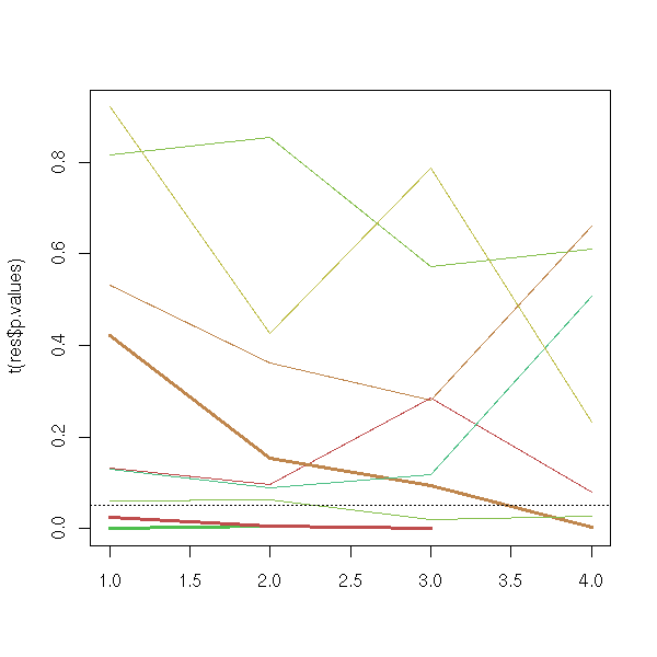
Exercise: improve the preceding function. Start with an empty set of variables; add them, one at a time, if their p-value is under 0.05, starting with the variables with the lowest p-value; when you run out aof variables to add, remove, one at a time, those whose p-value is larger that 0.05, startin with the variables with the highest p-value; when you run out of variables to remove, start adding them again; etc. What happens with the example above? What happens if we change the threshold?
Exercise: find, in the data provided with R or its packages, a data set with many variables (compared to the number of observations) and apply the methods presented above. What happens?
grep variable str_data |
  perl -p -e 's/^(.*\s)([0-9]+)(\s+variables:)/$2 $1$2$3/' |
  sort -n

library(ade4)
data(microsatt)
x <- microsatt$tab   # 18 observations, 112 variables, a lot of zeroes...
y <- x[,3]
x <- x[,-3]

For this example, we have 16 parameters for 18
observations: it does not work...

We can interpret this as follows.
The vector we wanted to predict is "almost" orthogonal to the
others.
No. It could be, but here it is not the case.

library(ade4)
data(microsatt)
x <- microsatt$tab   # 18 observations, 112 variables, a lot of zeroes...
y <- x[,3]
x <- x[,-3]
yn <- y/sqrt(sum(y*y))
xn <- t(t(x)/sqrt(apply(x*x, 2, sum)))
plot( sort(as.vector(t(yn) %*% xn)), type='h')
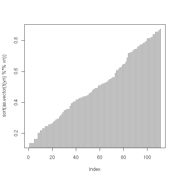
Actually, there are already a few functions to do this.
regsubsets (in the "leaps" package)
leaps      (in the "leaps" package -- prefer "regsubsets")
subset     (in the "car" package)
stepAIC    (in the "MASS" package)
Let us try them on our example.
d <- get.sample()
y <- d[,1]
x <- as.matrix(d[,-1])

library(leaps)
a <- regsubsets(y~x)
summary(a)
It yields (the "true" variables are 1, 3, 6, 7, 10):
Selection Algorithm: exhaustive
         X1  X2  X3  X4  X5  X6  X7  X8  X9  X10
1  ( 1 ) " " " " " " " " " " " " "*" " " " " " "
2  ( 1 ) " " " " "*" " " " " " " " " " " " " "*"
3  ( 1 ) " " " " "*" " " " " " " "*" " " " " "*"
4  ( 1 ) "*" " " "*" " " " " " " "*" " " " " "*"
5  ( 1 ) "*" " " "*" " " " " " " "*" "*" " " "*"
6  ( 1 ) "*" " " "*" " " " " " " "*" "*" "*" "*"
7  ( 1 ) "*" " " "*" " " " " "*" "*" "*" "*" "*"
8  ( 1 ) "*" " " "*" "*" " " "*" "*" "*" "*" "*"
The "subsets" function in the "car" packages can plot this.
library(leaps)
library(car)
get.sample <- function () {
  # Number of observations
  n <- 20
  # Number of variables
  m <- 10
  # Number of the variables that actually appear in the model
  k <- sample(1:m, 5)
  print(k)
  # Coefficients
  b <- rnorm(m); b <- round(sign(b)+b); b[-k] <- 0
  x <- matrix(nr=n, nc=m, rnorm(n*m))
  y <- x %*% b + rnorm(n)
  list(y=y, x=x, k=k, b=b)
}
d <- get.sample()
x <- d$x
y <- d$y
k <- d$k
b <- d$b
subsets(regsubsets(x,y), statistic='bic', legend=F)
title(main=paste(sort(k),collapse=', '))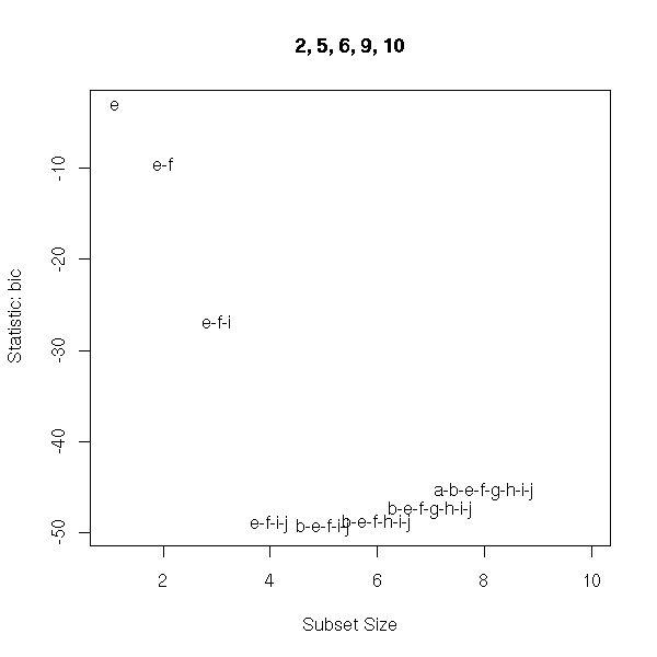
Let us also mention the "stepAIC" function, in the "MASS" package.
d <- data.frame(y=y,x)
r <- stepAIC(lm(y~., data=d), trace = TRUE)
r$anova

> r$anova
Stepwise Model Path
Analysis of Deviance Table

Initial Model:
y ~ X1 + X2 + X3 + X4 + X5 + X6 + X7 + X8 + X9 + X10

Final Model:
y ~ X1 + X3 + X4 + X5 + X7 + X10

  Step Df    Deviance Resid. Df Resid. Dev      AIC
1      NA          NA         9   18.62116 20.57133
2 - X9  1 0.007112768        10   18.62828 18.57897
3 - X6  1 0.037505223        11   18.66578 16.61919
4 - X2  1 0.017183580        12   18.68296 14.63760
5 - X8  1 0.098808619        13   18.78177 12.74309

> k
[1]  5 10  3  7  4
Let us compare with the theoretical model.
> summary(lm(y~x[,k]))
...
            Estimate Std. Error t value Pr(>|t|)
(Intercept)   0.2473     0.3023   0.818 0.426930
x[, k]1       1.7478     0.3330   5.249 0.000123 ***
x[, k]2       1.4787     0.2647   5.587  6.7e-05 ***
x[, k]3      -1.5362     0.4903  -3.133 0.007334 **
x[, k]4      -1.1025     0.2795  -3.944 0.001470 **
x[, k]5       1.6863     0.4050   4.164 0.000956 ***
Residual standard error: 1.27 on 14 degrees of freedom
Multiple R-Squared: 0.8317,     Adjusted R-squared: 0.7716
F-statistic: 13.84 on 5 and 14 DF,  p-value: 5.356e-05
> AIC(lm(y~x[,k]))
[1] 73.1798

> b
 [1]  0  0 -2  2  2  0 -1  0  0  2

> summary(lm(y~x[,c(1,3,4,5,7,10)]))
...
                           Estimate Std. Error t value Pr(>|t|)
(Intercept)                  0.1862     0.2886   0.645  0.52992
x[, c(1, 3, 4, 5, 7, 10)]1  -0.4408     0.2720  -1.620  0.12915
x[, c(1, 3, 4, 5, 7, 10)]2  -1.6742     0.4719  -3.548  0.00357 **
x[, c(1, 3, 4, 5, 7, 10)]3   1.5300     0.3953   3.870  0.00193 **
x[, c(1, 3, 4, 5, 7, 10)]4   1.7813     0.3159   5.639 8.07e-05 ***
x[, c(1, 3, 4, 5, 7, 10)]5  -1.0521     0.2664  -3.949  0.00167 **
x[, c(1, 3, 4, 5, 7, 10)]6   1.4903     0.2506   5.946 4.85e-05 ***
Residual standard error: 1.202 on 13 degrees of freedom
Multiple R-Squared:  0.86,      Adjusted R-squared: 0.7954
F-statistic: 13.31 on 6 and 13 DF,  p-value: 6.933e-05
> AIC(lm(y~x[,c(1,3,4,5,7,10)]))
[1] 71.50063
If we look at the p-values, we would like to remove X1, but if we look at the AIC, we would like to keep it...
TODO
The main problem of stepwise regression is that we are very likely to choose a bad model. An alternative is to this is select not one but several models. Then, we can compute the forecasts for each of those models and combine them, giving them a weight proportionnal to the likelihood of the model.
# We select a "good" regression model, using the BIC as a
# criterion, by starting from a model and adding or
# removing variables at random, if this improves the BIC.

# The second version also accepts models that are slightly
# worse, with a certain probability (high if the model is
# only slightly worse, low if it is really worse). We end
# up with a Markov chain that wanders in the space of all
# models, staying longer at models that are more
# probable. You can use this to average predictions over
# those models. This is called MCMC (Markov Chain Monte
# Carlo) or MCMCMC (Markov Chain Monte Carlo Model
# Combination).

# You can also change the "temperature", i.e., the
# probability that a worse model will be accepted, when
# the algorithm proceeds. If you end with a temperature
# equal to zero, you get a single solution, as with the
# steepest descent, but you are less likely to be stuck in
# a local minimum (this is called simulated annealing); if
# you decrease the temperature until 1, you get another
# MCMC, with a different burn-up period.

# For more details:
#   http://www.stat.washington.edu/raftery/Research/PDF/volinsky1997.pdf
#   http://www.research.att.com/~volinsky/bma.html
library(stats4)  # for BIC
bma.fit.model <- function (y, x, df) {
  # df: data.frame containing the data
  # y: name of the variable to predict
  # x: name of the predictive variables (vector of strings)
  if (length(x)==0) { x <- "1" }
  s <- paste("lm(", y, "~", paste(x, collapse="+"), ", data=df)")
  #cat(">", s, "\n")
  r <- eval(parse(text=s))
  BIC(logLik(r))
}
bma.neighbour <- function (model, variables) {
  # model:    vector containing the variables in the current model
  # variable: vector containing the names of all the variables among
  #           which we choose.
  model <- variables %in% model
  n <- length(model)
  i <- sample(1:n, 1)
  model[i] <- ! model[i]
  variables[ model ]
}
bma.steepest.descent <- function (y, x, df, N=1000) {
  # df: data.frame containing the data
  # y: name of the variable to predict
  # x: name of the predictive variables among which we
  #    shall choose
  # N: Number of iterations
  current.model <- character(0)
  current.bic <- bma.fit.model(y,current.model,df)
  for (i in 1:N) {
    new.model <- bma.neighbour(current.model, x)
    new.bic <- bma.fit.model(y, new.model, df)
    if (new.bic < current.bic) {
      current.bic <- new.bic
      current.model <- new.model
      cat("(", i, ") BIC=", current.bic, " ",
          paste(current.model,collapse=" "), "\n", sep="")
    } else {
      cat("(",i,") BIC=", new.bic, "\r", sep="")
    }
  }
  current.model
}
bma.mcmc.descent <- function (y, x, df, N=1000, temperature=1) {
  if (length(temperature)==1) {
    temperature <- rep(temperature,N)
  }
  res <- matrix(NA, nr=N, nc=length(x))
  colnames(res) <- x
  current.model <- character(0)
  current.bic <- bma.fit.model(y,current.model,df)
  for (i in 1:N) {
    new.model <- bma.neighbour(current.model, x)
    new.bic <- bma.fit.model(y, new.model, df)
    res[i,] <- x %in% new.model
    if ( current.bic - new.bic > temperature[i] * log(runif(1)) ) {
      current.bic <- new.bic
      current.model <- new.model
      cat("(", i, ") BIC=", current.bic, " ",
          paste(current.model,collapse=" "), "\n", sep="")
    } else {
      cat("(",i,") BIC=", new.bic, "\r", sep="")
    }
  }
  res
}

N <- 100
df <- data.frame(
  y = rnorm(N),
  x1 = rnorm(N),
  x2 = rnorm(N),
  x3 = rnorm(N),
  x4 = rnorm(N),
  x5 = rnorm(N)
)
df$y <- df$y + .1 * df$x1 + .5 * df$x3
bma.steepest.descent("y", setdiff(names(df),"y"), df)
r <- bma.mcmc.descent("y", setdiff(names(df),"y"), df)
apply(r[-(1:500),], 2, sum)
bma.mcmc.descent("y", setdiff(names(df),"y"), df, N=1000,
                 temperature=c(seq(20,1,length=500),  # Simulated annealing
                               seq(1,0,length=250),
                               rep(0,250)))

TODO: Explain what I am doing...
TODO: A prior (for the number of variables...)
TODO: Explain the danger of MCMC: we have to check that it
      actually converges. Typically: run several chains
      with different starting points, they should give the
      same results.
TODO: A few plots???
  barplot( apply(r[-(1:500),], 2, sum) )
  predictions with the "best" (wrong) model and
  predictions with the average model (but what do we plot?
  the error histograms? error2~error1?)

TODO: An example where it works...
True model: y ~ x1 + x2 + x3 but x1, x2 and x3 are not observed,
we only have x11 = x1 + noise1, x12 = x1 + noise2, etc.
The MCMC should alternate between x11 and x12, x21 and x22, etc.
You might also want to have a look at the BMA and ensembleBMA packages.
Other approaches try to combine models, not predictions -- for this, the models have to be expressed or transformed into a common framework.
Imagine you want to predict a quantitative variable y from other variables x1, ..., xn; you have tried several algorithms (say, logistic regression, stepwise logistic regression, decision trees, decision forests, support vector machines (SVM), neural networks) and you would like to compare them. You can easily measure how they fare on the learning sample, bit what will happen with new data? Indeed, if the model performs well on the training data, it might simply have overfitted the data and be completely useless -- there is a subtle tradeoff between the performance on the training sample and the ability to generalize.
TODO: a plot depicting this tradeoff.
performance in-sample      ~  model complexity
performance out-of-sample  ~  model complexity
(on the same plot)

set.seed(1)
n <- 20
x <- runif(n, -1, 1)
y <- 1 - x^2 + .2*rnorm(n)
X <- runif(10000, -1, 1)
Y <- 1 - X^2 + .2*rnorm(1000)
N <- n
res <- matrix(NA, nc=N, nr=2)
dimnames(res) <- list(
  c("In-sample error", "Out-of-sample error"),
  "Model complexity" = as.character(1:N)
)
r <- lm(y~x)
res[1,1] <- mean(abs(residuals(r)))
res[2,1] <- mean(abs(predict(r, data.frame(x=X)) - Y))
for (i in 2:N) {
  r <- lm(y ~ poly(x,i-1))
  res[1,i] <- mean(abs(residuals(r)))
  res[2,i] <- mean(abs(predict(r, data.frame(x=X)) - Y))
}

op <- par(mar=c(5,4,4,4))
ylim <- c(0, 1.5*max(res[1,]))
plot(res[1,], col="blue", type="l", lwd=3,
     ylim=ylim,
     axes=F,
     xlab="Model complexity",
     ylab="",
     main="In- and out-of-sample error")
axis(1)
axis(2, col="blue")
par(new=TRUE)
plot(res[2,], col="red", type="b", lwd=3,
     ylim=ylim,
     axes=F, xlab="", ylab="", main="")
axis(4, col="red")
mtext("In-sample error",     2, line=2, col="blue", cex=1.2)
mtext("Out-of-sample error", 4, line=2, col="red",  cex=1.2)
par(op)
A simple way of estimating the ability of a model to generalize is to cut the sample into two parts, use the first as a training set and the second as a test sample, to assess the model. To get a better idea, you can repeat this several times, with different partitions of the initial sample.
TODO: Example (take an example from "mlbench" and keep it
until the end of this section. Also choose a couple of
algorithms, say: logistic regression, stepwise logictic
regression, SVM and stick to them.)

for (i in data(package="mlbench")$results[,"Item"]) {
  do.call("data", list(i))
  cat(i, "\n")
  str(get(i))
}

# If we restrict ourselves to predicting a binary variable
str(Sonar)
str(PimaIndiansDiabetes)
str(Ionosphere)

library(mlbench)
data(Sonar)
glm( Class ~ ., data=Sonar, family="binomial")
Another way of estimating the quality of a model is the log-likelihood, i.e., the (conditionnal) probability of observing the data we have actually observed given the model -- however, if the model is sufficiently complex, i.e., if it has sufficiently many parameters, it can perfectly fit the learning sample. This prevents us from comparing models with a different number of parameters -- which is exactly what we want to do...
One way out of this problem is to compensate for an excessive number of parameters by adding a "penalty" to the log-likelihood, depending on the number of parameters. The AIC (Akaike Information Criterion) and the BIC (Bayesian Information Criterion) are examples of such penalized log-likelihoods.
TODO: Example
You might have a few qualms about the "number of parameters" used in the definition of the AIC or the BIC. Indeed, if you have two parameters, you can cheat and code them as a single number (just choose a bijection between R and R^2). But even without cheating, this poses a problem: how do we count the "number of variable" in a regression on the subset of variables? We have to somehow combine the number of initial variables (n) and the number of selected variables (k): do we consider that there are n parameters (some of which are zero)? do we use a boolean parameter for each variable telling us if it is retained or not (n+k parameters)? do we only count the retained variables (k parameters)? do we use a single discrete-valued variable to code the subset of retained variables (k+1 parameters)?
The notion of "number of variables" is fine for classical regression, but the problems we have just mentionned call for an other, more general notion, better suited to "machine learning algorithms", i.e., to algorithmic and not only statistical methods.
Enters the VC (Vapnik-Chervonenkis) dimension.
The situation is as follows: we have a qualitative variable y, quantitative variables x1, ..., xn neasured on a sample; we refer to (x1(i),...xn(i)) (without y) as an observation; we also have a classification algorithm f : (x,a) |---> f(x,a) that tries to predict y from x; here, "a" are the parameters of the classification algorithm, to be deternined (e.g., the coefficients of a regression, the weights of a neural network).
The classification algorithm f is said to shatter the observations o1,...,om if, for any training set (o1,y1),...,(om,ym) there exists a such that f(.,a) makes no mistakes on the training set. If you prefer formulas:
y \in Y   (Y is a finite set)
x \in R^n
a in |
f: X*A --> Y
f shatters (x1,...,xm) \in (R^n)^m iif
  \forall y1,...,ym \in Y
  \exists a \in A
  \forall i \in [1,m]
  f(xi, a) = yi
The VC dimension of the classification algorithm f is the largest number of points shattered by f. If you prefer formulas:
VC(f) = Max { m : \exists x1,...,xm \in R^n
                  such that x1,...,xn shatters f }
      = Max { m : \exists x1,...,xm \in R^n
                  \forall y1,...,ym \in Y
                  \exists a \in A
                  \forall i \in [1,m]
                  f(xi, a) = yi                  }
Examples:
VC(linear classifier, in dimension n) = n + 1
VC(SVM) = ???

TODO
The raison d'etre of the VC dimension is the following theorem:
Out-of sample error rate <= In-sample error rate +
                            sqrt( (VC*(1 + log(2N/VC)) - log(p/4)) / N )
with probability p, where N is the test sample size.
One can use this formula for "Structural Risk Minimization" (SRM) and choose the model with the lowest VC bound on the out-of-sample error rate -- this bound plays the same role as the AIC or the BIC.
TODO: plot
in-sample error  ~  model
VC bound on the out-of-sample error  ~  model
There is however a problem with this bound: it is extremely conservative -- your classification algorithm could well perform 100 times better...
As a conclusion, if you have to select a model among several, stick to the BIC (if you know how to compute it for your algorithm and if your data are well-behaved) or cross-validation.
For more details, check A. Moore's tutorials:
http://www.autonlab.org/tutorials/vcdim08.pdf
http://www.autonlab.org/tutorials/
If you want to choose a model from a reasonable set (say, a few dozen models), you can fit them all, compute some measure of model quality (AIC, BIC, cross-validation error, VC bound, etc.) and select the best one.
If the number of models is not reasonable (for instance, if you have 100 variables and want a model using a subset of them -- there are 2^100 of them), you can try various optimization algorithms, that wander through the space of all models (e.g., try to add or remove a variable to the current model and keep the new one if it is better, again and again, until you can no longer improve it -- this is a descent algorithm, but you could also use simulated annealing to avoid local extrema.
But sometimes, the number of models is not reasonable and the models are rather unwieldy: there can be no simple and obvious notion of a "nearby" model that would allow you to easily sample the space of all models. This is the case, for instance, if you want a non-linear model: your space of models could be "all the formulas one can obtain from the predictive variables, the basic arithmetic operations (+ - * /) and a few selected functions (sin, exp, log)".
Such a formula can be represented by a tree. For instance,
         sqrt( 1 - x1 * x3 )
1.17 * -----------------------
        exp( sin( x1 / x2 ) )
can be represented as
          *
         / \
        /   \
       /     \
     1.17     /
             / \
            /   \
           /     \
        sqrt     exp
         |        |
         |        |
         |        |
         -       sin
         |      /  \
         |     /    \
         |    /      \
         1   *       /
            / \     / \
           /   \   /   \
          x1   x3 x1   x2
The Lisp programmers amoung you would represent this as
(* 1.17
   (/ (sqrt (- 1 (* x1 x3)))
      (exp (sin (/ x1 x3)))))
Contrary to waht it seems, this complex structure does not rule out classical local search algorithms: all we need is a notion of a "nearby" formula or "nearby" tree. Indeed, one can get a tree near a given one by applying one of the following "mutations": replace a node (an operator) by another, of the same arity; replace a leaf; select a subtree and replace it by a random tree; insert a node (if its arity if not one, complete it with random trees); delete a node; splice the root.
One can go one step further and use genetic algorithms: contrary to local search methods, where we have a single current candidate model, we have a pool (or "population") of models (one or two hundreds) and we go from one generation to the next by mutating and pairing the models. Besides the mutations, we also need a way to combine two parent models into a child model; this is called cross-over and can be done as follows: select a subtree in both parents and interchange them.
TODO: Implementation?
(I am not sure R is the language of choice if you want to
play with trees).
See also:
http://www.olsen.ch/research/workingpapers/gpForVolatility.pdf
http://www.olsen.ch/research/307_ga_pase95.pdf
Generalizations:
- Respect the type of the operators (in programming language parlance, the signature of the functions), i.e., take into account wether the functions take as arguments and return arbitrary reals, reals in the interval [0,1], positive numbers, boolean values, etc.
- Do not use genetic algorithms for the constants, but use classical optimization algorithms;
- Take into account the possibility of non-relevant peaks in the BIC landscape, e.g., by penalizing the BIC according to the number of individuals around or by clustering the individuals, thereby creating subpopulations;
- Be creative and use other kinds of operators, for instance, exponential moving averages (in finance, people feed very long irregular time series to genetic algorithms) or boolean operators (< & | ifelse, e.g., to create trading rules).
The "dr" package provides several dimension reduction algorithms.
library(help=dr)
xpdf /usr/lib/R/library/dr/doc/drdoc.pdf
TODO: (understand and) explain those algorithms: sir, save, phd. (the PDF file above is not clear).
sir    Sliced Inverse Regression
save   Sliced Average Variance Estimation
phd    Principal Hessian Direction
TODO: an example, with a few plots... (take another example, not that from the manual...)
# From the manual
library(dr)
data(ais)

# The data
op <- par(mfrow=c(3,3))
for (i in names(ais)) {
  hist(ais[,i], col='light blue', probability=T, main=i)
  lines(density(ais[,i]),col='red',lwd=3)
}
par(op)

# Their logarithm
op <- par(mfrow=c(3,3))
for (i in names(ais)) {
  x <- NA
  try( x <- log(ais[,i]) )
  if( is.na(x) | any(abs(x)==Inf) ){
    plot.new()
  } else {
    hist(x, col='light blue', probability=T, main=i)
    lines(density(x),col='red',lwd=3)
  }
}
par(op)

# Dimension reduction
r <- dr(LBM ~ Ht + Wt + log(RCC) + WCC, data=ais, method="sir")
plot(r)
r
summary(r) # TODO: mention the tests for the dimension
SVM appear, for instance, in the following situation.
Genetics can be used to assess a risk in a patient. If we know the mecanisms behind a given pathology, if we know what genes are involved (i.e., what genes are over- or under-expressed in that pathology, or what mutations trigger the disease), we can perform the tests. But often, we do not know the mecanisms of the pathology -- yet. However, we can still hope to come to a conclusion by performing tests "at random". We take a few dozen patients (or a few hundred: those tests are very expensive), whose condition is known (for instance, by invasive tests, such as post-mortem examinations) and we look for the presence/absence, or for the expression of tens of tousands of genes (this can be done on a small piece od glass called a "micro-chip" or a "micro-array"). And we want to predict the patient's condition (wether he has the disease) from the genes.
You have noticed the problem: there are too many variables. (As a rule of thum, you should have (at least) ten times more parameters to estimate than observations -- here, it could be 100 times less...)
First idea: restrict yourself to 20 variables, chosen on the basis of prior knowledge.
Second idea: restrict yourself to 20 variables, the 20 best. The is the variable selection, that we have already presented.
Third idea: In the case the variable to predict is qualititive (as in our example), the problem is to find a hyperplane separating two clouds of points. Instead of looking for a hyperplane, i.e., an affine function f so that f>0 iif the patient is affected (if there are really many variables, there is a wealth of such hyperplanes), we can look for a thick hyperplance, i.e., an affine function f so that f > a iif the patient is affected and f < -a iif the patient is not affected, with a as large as possible.
Actually, the SVM method is more general: we first increase the dimension, to allow for non-linear effects (for instance, we could map a 2-dimensional vector space to a 5-dimensional vector space by (x,y) --> (x,y,x^2,y^2,x*y)) and only then look for a thick separating hyperplane.
The algorithm is as follows.
1. Find a separating thick hyperplane, as thick as possible. This is a simple Lagrange multipliers problem -- it can also be seen as a quadratic programming problem. We have a Lagrange multiplier for each point: if the multiplier is zero, the points does not play any role (it is in the midst of the cloud of points, it is far away from the separating hyperplane); if the multiplier is non-zero, we say it is a "support vector". Those points will "touch" the thick hyperplane, they will limit its thickness -- actually, you can even forget the other points
2. If it does not work, increase the dimension. You could try various embeddings, such as (x,y) |---> (x,x^2,x*y,y^2), but actually, we can simply change the "hyperplane" equation (well, it will no longer be a hyperplane) by replacing the scalar product used to define it by a kernel, such as K(x,y) = ( <x,y> + a )^b or K(x,y) = exp( -a Norm(x-y)^2 ). If you use algorithms that do not use coordinates but just scalar products, this trick (the "kernel trick") allows you to increase the dimension without having to compute the actual coordinates.
3. You can also accept that certain points end on the "wrong" side of the hyperplane, with a penality.
n <- 200
x <- rnorm(n)
y <- rnorm(n)
u <- sqrt(x^2+y^2)
u <- ifelse( u<.5*mean(u), 1, 2)
plot(y~x, col=u, pch=15)
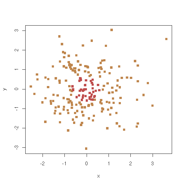
help.search("svm")
help.search("support vector machine")
library(e1071)
library(help=e1071)
?svm

library(e1071)
u <- factor(u)
r <- svm(u~x+y)
{
  # The "plot.svm" calls "browser()": Why???
  # (I use it when I debug my code, it is probably the
  # same for them.)
  # And then it crashes...
  # (e1071 version 1.3-16, 1.3-16)
  browser <- function () {}
  try(  plot(r, data.frame(x,y,u), y~x)  )
}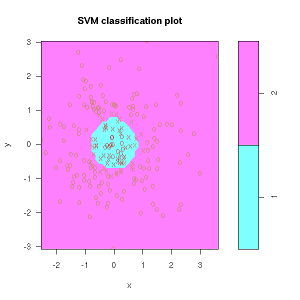
n <- 200
x <- runif(n, -1,1)
y <- runif(n, -1,1)
u <- abs(x-y)
u <- ifelse( u<.5*mean(u), 1, 2)
plot(y~x, col=u, pch=15)
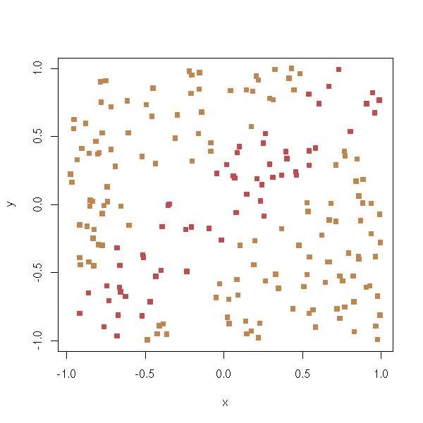
u <- factor(u)
r <- svm(u~x+y)
{
  browser <- function () {}
  try(  plot(r, data.frame(x,y,u), y~x)  )
}
If you want to seriously use SVMs, you will try various values for the "cost" and "gamma" parameters, and you will select the best with, for instance, a cross-validation.
SVM can be generalized:
To distinguish between more than two classes, you can consider the classes two at a time and then use a majority rule to forecast the class of a new observation.
Alternatively, you can also try to distinguish a class against the union of all the other classes; do that for each class; then use a majority rule for prediction.
One can also use SVM to "distinguish between a single class". It sounds odd, but it allows you to spot outliers.
you can also use SVMs for regression. In linear regression, you are looking for a hyperplane "near" most of the points; with SVMs, you will be looking for a thick hyperplane, as thin as possible, that contains all the observations. It is the same Lagrange multiplier problem as above, with all the inequalities reversed.
There is a dual way of interpreting these methods: take the median hyperplane of the segment joining the two nearest points in the convex hull of both clouds of points. If the convex hull intersect, replace them with "reduced convex hulls" (still defined as the set of barycenters of the points, but with a restriction on the coefficients: for instance, we ask that they be all under 0.5, so as not to give too much importance to an isolated point).
For more details, more examples and a comparison of SVMs and regression trees, see
/usr/lib/R/library/e1071/doc/svmdoc.pdf
For other details:
http://bioconductor.org/workshops/Heidelberg02/moldiag-svm.pdf
http://www.kernel-machines.org/
http://www.csie.ntu.edu.tw/~cjlin/papers/ijcnn.ps.gz
http://www.acm.org/sigs/sigkdd/explorations/issue2-2/bennett.pdf
http://www.csie.ntu.edu.tw/~cjlin/papers/libsvm.ps.gz
Exercise: use an SVM in the situation described in the introduction (microarrays).
TODO: explain (understand?) what follows. Is it finished???
library(help=sma)
library(help=pamr)
library(e1071)
library(sma)
data(MouseArray)
# Mice number 1, 2 and 3: control
# Number 4, 5, 6: treatment
m <- t(mouse.lratio$M)
m <- data.frame( mouse=factor(c(1,1,1,2,2,2)), m)
# r <- svm(mouse~., data=m, na.action=na.omit, kernel="linear")
# Out of memory...
m <- m[,1:500]
r <- svm(mouse~., data=m, na.action=na.omit, kernel="linear")
TODO: finish this.
In particular: how do we read the result?
Forecast;
m <- t(mouse.lratio$M)
m <- m[,!is.na(apply(m,2,sum))]
m <- data.frame( mouse=factor(c(1,1,1,2,2,2)), m)
m <- m[,1:500]
m6 <- m[6,]
m <- m[1:5,]
r <- svm(mouse~., data=m,
na.action=na.omit, kernel="linear")
predict(r,m6) # 1 instead of 2...
r <- svm(mouse~., data=m,
na.action=na.omit)
predict(r,m6) # 1 instead of 2...
# One could expect that kind of error:
library(cluster)
m <- t(mouse.lratio$M)
m <- m[,!is.na(apply(m,2,sum))]
plot(hclust(dist(m)))
rm(m,m6,r)
Generalized Additive Models (GAMs) appear when you try to describe a non-linear situation with a large number of variables.
If the model were linear, the number of variables would be reasonable, but in a non-linear situation, it explodes...
For a linear model, we would write
Y = b0 + b1 x1 + b2 x2 + ... + bn xn.
where the bi are numbers. There are n+1 parameters to estimate.
A non-linear model would be
Y = f(x1,x2,...,xn)
where f is any function. Even if you restrict the shape of the function f, say, a polynomial of degree 2, the dimension of the space of such functions grows to fast (here, 1+n+n(n+1)/2).
Side note: at school, one studies polynomials of one variable, but not polynomial of several variables. One of the reason is that dimension -- actually, you can give a geometric interpretation of the computations you do with polynomials: with one variable, you are in a straight line, and the geometry of the straight line is, well, straightforward; with two variables, you are in the plane, you can study curves, which can be more intricate; the more variables you have, the more complicated the geometry. This is called algebraic geometry. End of the side note.
A generalized additive model is
Y = a + f1(x1) + f2(x2) + ... + fn(xn)
where the fi are arbitrary functions (you will estimate them as you want: splines, kernel, local regression, etc.). The important point is that they are functions of one variable: they are not too complex.
Of course, all the functions R^n --> R cannot be written like that: but we have a lot of them and most of the time this will be sufficient. But a big problem lurks behind this simplification: we completely forget potential interactions between variables. Non-linearity or integration, you will have to choose. (Well, actually, if you think there is an interaction between two of your variables, you will include this interaction -- but just this one --; the model then becomes y = a + f(x1,x2) + f3(x3) + ... + f(xn).)
The algorithm used to find those functions is iterative. If we forget the constant, it would be:
1. Take a first estimation of the fi, say, as constants, from a linear regression.
2. For all k, define fk as the local regression of
Y - Sum(fj(xj)) ~ Xk j!=k
3. Iterate ultil convergence.
If you do not forget the constant:
1. alpha <- mean(y)
f[k] <- 0
2. f[k] <- Smoother( Y - alpha - Sum(fj(xj)) )
j!=k
3. f[k] <- f[k] - 1/N * Sum fk(xik)
i
4. Goto 2 until the f[k] no longer change.You can generalize this algorithm by adding interaction terms, when needed: fij(xi,xj), etc.
You can also ask that some of those functions have a predetermined form, e.g., that they be linear.
One can show that this algorithm actually minimizes a penalized sum of squares.
Variant: You can generalize this method to logistic or Poisson regression (it is then interpreted with a penalized log-likelihood), but the algorithm is a bit different (a mixture of backfitting and IRLS). For a multilogistic regression, it is even more complicated.
You can also interpret the Generalized Additive Model as the quest for the best transformation of the predictive variables so that the linear model be valid.
Remark: as always, we assume that the variable to predict is gaussian -- it is significantly non gaussian, we shall transform it. For the predictive variables, it may not be that important, but (to avoid numeric instability) they should have the same order of magnitude (I think).
Let us now see how to do all this with R.
TODO library(mgcv) ?gam n <- 200 x1 <- runif(n,-3,3) x2 <- runif(n,-3,3) x3 <- runif(n,-3,3) f1 <- sin; f2 <- cos; f3 <- abs; y <- f1(x1) + f2(x2) + f3(x3) + rnorm(n) pairs(cbind(y,x1,x2,x3)) # Nothing really visible...
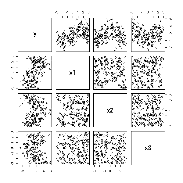
library(mgcv) r <- gam(y~s(x1)+s(x2)+s(x3)) x <- seq(-3,3,length=200) z <- rep(0,200) m.theoretical <- cbind(f1(x),f2(x),f3(x)) m.experimental <- cbind( predict(r, data.frame(x1=x,x2=z,x3=z)), predict(r, data.frame(x1=z,x2=x,x3=z)), predict(r, data.frame(x1=z,x2=z,x3=x)) ) matplot(m.theoretical, type='l', lty=1) matplot(m.experimental, type='l', lty=2, add=T)
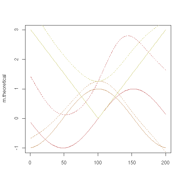
It is difficult to compare, because the curves are shifted...
zero.mean <- function (m) {
t(t(m)-apply(m,2,mean))
}
matplot(zero.mean(m.theoretical),
type='l', lty=1)
matplot(zero.mean(m.experimental),
type='l', lty=2, add=T)
title(main="GAM")
legend(par('usr')[2], par('usr')[3],
xjust=1, yjust=0,
c('theoretical curves', 'experimental curves'),
lty=c(1,2))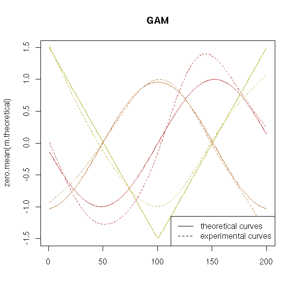
op <- par(mfrow=c(2,2))
for (i in 1:3) {
plot(r, select=i)
lines(zero.mean(m.theoretical)[,i] ~ x,
lwd=3, lty=3, col='red')
}
par(op)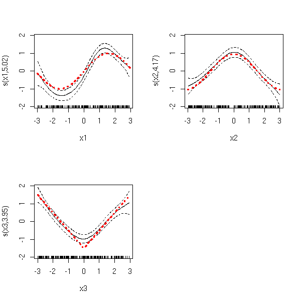
res <- residuals(r) op <- par(mfrow=c(2,2)) plot(res) plot(res ~ predict(r)) hist(res, col='light blue', probability=T) lines(density(res), col='red', lwd=3) rug(res) qqnorm(res) qqline(res) par(op)

op <- par(mfrow=c(2,2)) plot(res ~ x1) plot(res ~ x2) plot(res ~ x3) par(op)
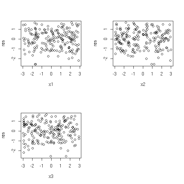
TODO: refer to other documents, URLs... TODO: "thin-plate regression spline" ???
TODO: Other functions to fit GAMs:
library(mda) ?bruto # Gaussian GAM library(help=gss) ?glm # ???
TODO: What criterion is used?
GCV ???
It is a means of predicting a qualitative binary variable with many (quantitative or qualitative) variables, with no linearity assumption whatsoever.
The algorithm is the following. Choose one of the variables and a cutpoint so as to maximize some statistical criterion; iterate until there are only a few (20 to 50) observations in each class. The result can be seen as a tree. prune that tree (for instance, compare with other (bootstrap) samples; or find the number of nodes so that the tree built from 90% of the data give the best possible results on the remaining 10%).
library(rpart) data(kyphosis) r <- rpart(Kyphosis ~ ., data=kyphosis) plot(r) text(r)

The first application is obtaining a decision tree, that can predict a result with few variables, i.e., with few tests (for instance, in emergency medicine).
Another application is the study of missing values.
library(Hmisc) ?transcan
It is VERY important to prune the tree, otherwise, you get a tree that describes the sample and not the population.
TODO: plot
The method can be generalized to predict a "counting variable" (Poisson regression).
This method is not very stable: a similar sample can give a completely different tree. However, you can reduce the variance of the result with the bagging method. See also MART.
We want to predict a binary variable Y from quantitative variables, by looking for boxes in the space of predictive variables in which we have often Y=1. The algorithm is the following.
1. Take a box (i.e., a part of the space delimited by hyperplanes parallel to the axes), containing all the data points. 2. Reduce it in one dimension so as to increase the proportion of points with Y=1. 3. Go back to 2, so that the box contains sufficiently few misclassified points. 4. Try to enlarge the box. 5. Remove the points from this box. 6. Start again, until there are no more points. 7. As always, prune the result, so as to avoid overfit.
We end up with a bunch of boxes, each of which can be seen as a rule. This is actually a variant of Regression Trees (CART): with regression trees, each node of the tree is a rule with exactly one variable and one equality; with PRIM, we still have a tree, its nodes are rules, but rule is made of several inequalities of the form X_i < a or X_i > a.
Apparently, this algorithm is not implemented in R.
help.search('PRIM')
help.search('bump')There are out-of-memory implementations (i.e., implementations that do not put all the data in memory): TurboPRIM.
One idea, to increase the quality on an estimator (a non-linear and unstable one, e.g., a regression tree) is simply to compute its "mean" on several bootstrap samples.
For instancem the result of forecast by a regression tree is usually a class (1, 2, ..., or k): we replace it by a vector (0,0,...,0,1,0,...,0) (put "1" for the predicted class, 0 for the others) and we take the average of those vectors -- we do not get a single class, but a probability distribution (bayesian readers will prefer the words "posterior distribution").
Remark: the structure of the estimator is lost -- if it was a tree, you get a bunch of trees (a forest), whose predictions are more reliable, but which is harder to interpret.
Remark: This idea has no effect whatsoever with linear estimators: they commute with the mean.
Remark: in some cases, the auelity of the estimator can worsen.
In the following example, the forecasts are correct 99% of the time.
library(ipred)
do.it <- function (formula, data, test) {
r <- bagging(formula, data=data, coob=T,
control=rpart.control(xval=10))
p2 <- test$Class
p1 <- predict(r,test)
p1 <- factor(p1, levels=levels(p2))
res1 <- sum(p1==p2) / length(p1)
# Only with the trees
r <- bagging(formula, data=data, nbagg=1,
control=rpart.control(xval=10))
p2 <- test$Class
p1 <- predict(r,test)
p1 <- factor(p1, levels=levels(p2))
res2 <- sum(p1==p2) / length(p1)
c(res1, res2, res1/res2)
}
# An example from "mlbench" (it is a collection of such
# examples)
library(mlbench)
data(Shuttle)
n <- dim(Shuttle)[1]
k <- sample(1:n,200)
do.it(
Class ~ .,
data = Shuttle[k,],
test = Shuttle[-k,]
) # Idem, 99.5%
rm(Shuttle)
data(Vowel)
n <- dim(Vowel)[1]
k <- sample(1:n,200)
do.it(
Class ~ .,
data = Vowel[k,],
test = Vowel[-k,]
) # Better: 47% instead of 36%
rm(Vowel)You can interpret the bagging method as an alternative to the maximum likelihood method: to estimate a parameter, the Maximum Likelihood Method looks at the distribution of this parameter and chooses its mode; Bagging, on the other hand, uses simulations to estimate this distribution (it is a randomized algorithm) and selects its mean.
See also:
/usr/lib/R/library/ipred/doc/ipred-examples.pdf
This is very similar to bagging (we compute an estimator on several bootstrap samples), but the bootstrap samples are not taken at random: they are selected according to the performance of the previous estimators. Usually, we simply assign a weight (a probability of appearing in the next bootstrap sample) to each observations according to the preceding results.
Usually, it works quite well, better that the bagging -- but in some cases, the estimator can worsen...
TODO: with R???
The methods presented above, bagging and boostring, replace an estimator by a set of estimators. We then use these families of estimators. All the estimators of a given family are of the same kind (say, all are trees, or all are neural networks).
But nothing prevents you from mixing completely different estimators.
TODO: examples (tree + linear regression?)
You can also use those methods for non-supervised classification (i.e., when you try to find classes in your sample, without any "training set" to hint at the rules to form those classes).
TODO: examples
Again, this is very similar to the bagging: we build regression trees on bootstrap samples, nut at each node of each tree, we do not use all the variables, but just a small (random) subset of variables. It can be seen as a "noisy" variant of bagging.
Here is an example (three or four minutes of computation -- there are 500 trees...).
library(randomForest)
do.it <- function (formula, data, test) {
r <- randomForest(formula, data=data)
p2 <- test$Class
p1 <- predict(r,test)
p1 <- factor(p1, levels=levels(p2))
res1 <- sum(p1==p2) / length(p1)
# Only with the trees
r <- bagging(formula, data=data, nbagg=1,
control=rpart.control(xval=10))
p2 <- test$Class
p1 <- predict(r,test)
p1 <- factor(p1, levels=levels(p2))
res2 <- sum(p1==p2) / length(p1)
c(res1, res2, res1/res2)
}
library(mlbench)
data(Vowel)
n <- dim(Vowel)[1]
k <- sample(1:n,200)
do.it(
Class ~ .,
data = Vowel[k,],
test = Vowel[-k,]
) # From 42% to 67%
rm(Vowel)It is better than bagging (with the same sample, we go from 42% to 45% of good answers).
Actually, the "randomForest" function is a little more verbose.
> r <- randomForest(Class~., data=Vowel)
> r
Call:
randomForest.formula(x = Class ~ ., data = Vowel[k, ])
Type of random forest: classification
Number of trees: 500
No. of variables tried at each split: 3
OOB estimate of error rate: 26%
Confusion matrix:
hid hId hEd hAd hYd had hOd hod hUd hud hed class.error
hid 11 3 0 0 0 0 0 0 0 3 0 0.3529412
hId 2 11 1 0 0 0 0 0 1 0 0 0.2666667
hEd 0 2 6 2 0 0 0 0 0 0 2 0.5000000
hAd 0 0 0 20 0 1 0 0 0 0 1 0.0909091
hYd 0 0 0 0 23 2 0 0 0 0 1 0.1153846
had 0 0 0 2 5 7 0 0 0 0 1 0.5333333
hOd 0 0 0 0 2 0 13 1 1 0 0 0.2352941
hod 0 0 0 0 0 0 2 11 1 0 0 0.2142857
hUd 0 0 0 0 0 0 2 2 16 2 0 0.2727273
hud 1 0 0 0 0 0 0 1 2 15 0 0.2105263
hed 0 0 0 0 2 2 0 0 2 0 15 0.2857143First, we remark that the error rate is optimistic (26% instead of 33% -- and the oob bootstrap is supposed to be pessimistic...).
We also get the confusion matrix, that gives the "distances" between the classes: we can use it to plot the classes in the plane, with a Distance Analysis algorithm (MDS (MultiDimensional Scaling), etc. -- we have already mentionned this).
library(randomForest) library(mlbench) library(mva) data(Vowel) r <- randomForest( Class ~ ., data = Vowel, importance = TRUE ) # Trois minutes... m <- r$confusion # We have a confusion matrix instead of a distance matrix. # We try to tweak the matrix to get something that looks # like a distance matrix -- this might not be the best way # to proceed. m <- m[,-dim(m)[2]] m <- m+t(m)-diag(diag(m)) n <- dim(m)[1] m <- m/( matrix(diag(m),nr=n,nc=n) + matrix(diag(m),nr=n,nc=n, byrow=T) ) m <- 1-m diag(m) <- 0 mds <- cmdscale(m,2) plot(mds, type='n') text(mds, colnames(m)) rm(Vowel)

We also have the importance of each of the predictive variables.
> r$importance
Measure 1 Measure 2 Measure 3 Measure 4
V1 178.94737 16.674731 0.9383838 0.4960153
V2 563.15789 38.323021 0.9222222 1.0000000
V3 100.00000 13.625267 0.8343434 0.4212575
V4 200.00000 23.420278 0.8909091 0.5169644
V5 321.05263 26.491365 0.8959596 0.5819186
V6 189.47368 20.299312 0.8828283 0.5022913
V7 84.21053 10.596949 0.7777778 0.3544800
V8 110.52632 16.071039 0.8454545 0.4107499
V9 47.36842 10.219346 0.8424242 0.3301638
V10 63.15789 8.857154 0.8292929 0.3274473TODO: explain/understand.
Graphically, this suggests that we only consider V2, or V2 and V5, or even V2, V5 and V1.
op <- par(mfrow = c(2,2))
m <- r$importance
n <- dim(m)[1]
for (i in 1:4) {
plot(m[,i],
type = "h", lwd=3, col='blue', axes=F,
ylab='', xlab='Variables',
main = colnames(r$importance)[i] )
axis(2)
axis(1, at=1:n, labels=rownames(m))
# The two highest values in red
a <- order(m[,i], decreasing=T)
m2 <- m[,i]
m2[ -a[1:2] ] <- NA
lines(m2, type='h', lwd=5, col='red')
}
par(op)
In the examples, we have stressed classification trees, but it also works with regression trees.
You can also use random forests to detect outliers.
TODO: finish reading the article in Rnews_2002-3.pdf http://cran.r-project.org/doc/Rnews/Rnews_2002-3.pdf (at the end: ROC)
See:
Rnews_2002-3.pdf http://cran.r-project.org/doc/Rnews/Rnews_2002-3.pdf TODO: I often speak of "regression trees", but I have only defined "classification trees". What is a "regression tree"? MARS?
TODO: move this section to a better location.
TODO: find real data with one (or two) group(s) of outliers.
Here, we simply ask the computer to try and find classes in the data. If he puts most of the data in a class and the rest in a few isolated classes, you should worry.
(Of course, if you have several variables, you first look at them one at a time, and only then all together.)
TODO: idem with hiearchical classification. should we get a balanced tree?
Surprisingly, you cam also use supervised learning algorithms. The idea is to put all the data in the same class and add random (uniformly distributed) data, in a second class. Then, we ask the computer to try to predict the class from the data. Observations from the first class but misclassified as elements of the second are potential outliers.
The "uniform distribution" is arbitrary and may not be a good choice. If you have already considered 1-dimensional problems and focus on outliers that are only revealed when you look at the data in higher dimensions, you can replace this uniform distribution by sampling independantly in each variable.
TODO: an example...
TODO: recall what a neural net is...
You can use neural nets for regression (i.e., to forecats a quantitative variable) or for supervised classification (i.e., to forecats a qualitative variable).
If we again our vowel recognition example, we get around 6% of good results (between 55% and 65%).
library(nnet)
do.it <- function (formula, data, test, size=20) {
r <- nnet(formula, data=data, size=size)
p2 <- test$Class
p1 <- predict(r,test)
nam <- colnames(p)
i <- apply(p1,1,function(x){order(x)[11]})
p1 <- nam[i]
p1 <- factor(p1, levels=levels(p2))
res1 <- sum(p1==p2) / length(p1)
res1
}
library(mlbench)
data(Vowel)
n <- dim(Vowel)[1]
k <- sample(1:n,200)
do.it(Class~., data=Vowel[k,], test=Vowel[-k,])
TODO
library(deal) demo(rats) TODO: look in /usr/lib/R/library/deal/demo/ hiscorelist <- heuristic(newrat, rats.df, rats.prior, restart = 10, degree = 7, trace = TRUE)
We are again in a regression setup: we want to predict a quantitative variable Y from quantitative variables X. To this end, we try to write Y as a linear combination of functions of the form (Xj-t)_+ or (t-Xj)_+, where Xj is one of the variables and t=xij is one of the observations. This is very similar to regression trees, but the forecasts are piecewise linear instead of piecewise constant.
The algorithm is the following (it is a regression, where the predictive variables are of the form (Xj-t)_+ and (t-Xj)_+ -- we do not take all these variables (there would be too many), but just a subset of them).
1. Start with a single, constant, function. 2. Compute the coefficients of the model. For the first iteration, it is simply Y ~ 1. 3. Add the pair of functions (Xj-t)_+, (t-Xj)_+ to the set of predictive variables, choosing Xj and t=xij so as to reduce the error as much as possible. 4. Go to 2. 5. Do not forget to prune the resulting tree! (as for regression trees or classification trees)
You can generalize this idea to logistic regression, multiple logistic regression, etc. (in those cases, you no longer use least squares to find the coefficients, but maximum likelihood).
In R, you can use the "mars" function from the "mda" package.
Let us consider the following example.
library(mda) library(mlbench) data(BostonHousing) x <- BostonHousing x[,4] <- as.numeric(x[,4]) pairs(x)
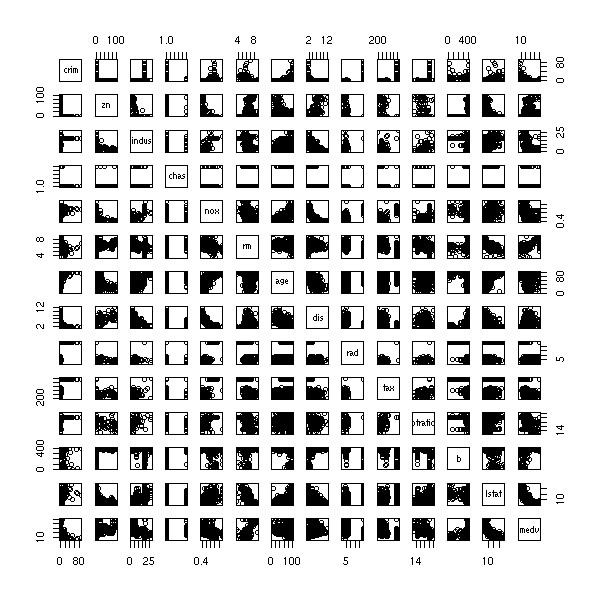
The variables seem very well suited to the methos: some have two "humps" -- and the very idea of the MARS algorithm is to separate such humps -- we should end with gaussian-looking variables.
op <- par(mfrow=c(4,4))
for (i in 1:14) {
hist(x[,i],probability=T,
col='light blue', main=paste(i,names(x)[i]))
lines(density(x[,i]),col='red',lwd=3)
rug(jitter(x[,i]))
}
hist(log(x[,1]),probability=T,
col='light blue', main="log(x1)")
lines(density(log(x[,1])),col='red',lwd=3)
rug(jitter(log(x[,1])))
par(op)
op <- par(mfrow=c(4,4))
for (i in 1:14) {
qqnorm(x[,i], main=paste(i,names(x)[i]))
qqline(x[,i], col='red')
}
qqnorm(log(x[,1]), main="log(x1)")
qqline(log(x[,1]), col='red')
par(op)
We take the logarithm of the variable to predict, becaus it is really far from gaussian (we leave the others alone: MARS will separate their humps and they should, afterwards, look normal). (At fisrt, I had not transformed it -- the results were extremely poor: the forecast error was as large as the the standard deviation of the variable...)
x[,1] <- log(x[,1])
n <- dim(x)[1]
k <- sample(1:n, 100)
d1 <- x[k,]
d2 <- x[-k,]
r <- mars(d1[,-1],d1[,1])
p <- predict(r, d2[,-1])
res <- d2[,1] - p
op <- par(mfrow=c(4,4))
plot(res)
plot(res~p)
for (i in 2:14) {
plot(res~d2[,i])
}
par(op)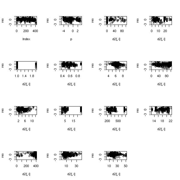
op <- par(mfrow=c(2,2))
qqnorm(r$fitted.values, main="fitted values")
qqline(r$fitted.values)
hist(r$fitted.values,probability=T,
col='light blue', main='fitted values')
lines(density(r$fitted.values), col='red', lwd=3)
rug(jitter(r$fitted.values))
qqnorm(res, main="residuals")
qqline(res)
hist(res, probability=T,
col='light blue', main='residuals')
lines(density(res),col='red',lwd=3)
rug(jitter(res))
par(op)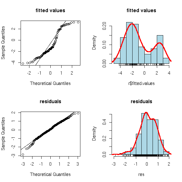
If we compare with a naive regression, it is slightly better.
> mean(res^2) [1] 0.6970905 > r2 <- lm(crim~., data=d1) > res2 <- d2[,1] - predict(r2,d2) > mean(res2^2) [1] 0.7982593
A naive regression with anly the "hunched" variables (bad idea@ the other variables bring som important information):
> kk <- apply(r$cuts!=0, 2, any) > kk <- (1:length(kk))[kk] > kk <- c(1, 1+kk) > r3 <- lm(crim~., data=d1[,kk]) > res3 <- d2[,1] - predict(r3,d2) > mean(res3^2) [1] 0.7930023
If we try to select the variables:
> library(MASS) > r4 <- stepAIC(lm(crim~., data=d1)) > res4 <- d2[,1]-predict(r4,d2) > mean(res4^2) [1] 0.8195915
(You can try many other methods...)
This is similar to CART, with the following differences. The nodes of the tree are probabilistic. The nodes depend on a linear combinaition of the predictive variables, not of a single variable. We perform a linear regression at each leaf (with CART, we assign a constant to each leaf). There is no algorithm to find the structure of the tree: you have to choose it yourself.
TODO: with R?
TODO
heuristic(deal) Heuristic greedy search with random restart Title: Learning Bayesian Networks with Mixed Variables tune.rpart(e1071) Convenience tuning functions
??? TODO
??? TODO
TODO: put this somewhere else -- it should be with ridge regression, partial least squares, etc.
Principal component Analysis is a simple and efficient means of reducing the dimensionality of a data set, or reducing the number of variables one will have to look at but, it the context of regression, it misses a point: in principal component regression, where one tries to predict or explain a variable y from many variables x1, ..., xn, one computes the PCA of the predictive variables x1,...,xn, and regresses y against the first components -- but one does not take the variable to predict into account! In other words, we select non-redundant variables, that account for the shape of the cloud of points in the x variables, instead of selecting non-redundant variables with some power to predict y.
This is the same problem that leads to Partial Least Squares (PLS). Supervised principal components are much easier to understand, though. The algorithm goes as follows:
Compute the principal components of those of the predictive variables that are the most correlated with the variable to predict y (using some threshold, chosen by cross-validation). Regress y against the first principal components.
Well, the actual algorithm is slightly more complicated: one does not directly us the correlation to select the variables. For more details, see:
http://www-stat.stanford.edu/~tibs/ftp/spca.pdf http://www-stat.stanford.edu/~tibs/superpc/tutorial.html
In R, this method is available in the "superpc" package and can accomodate classical or survival regression.
TODO: Example...
library(superpc)
# Some simulated data
n <- 50 # Number of observations (e.g., patients)
m <- 500 # Number of values to predict
p <- 1000 # Number of variables or "features" (e.g., genes)
q <- 20 # Number of useful variables
x <- matrix( rnorm((n+m)*p), nr=n+m )
z <- svd(x[,1:q])$u
y <- 1 - 2 * z[,1]
d <- list(
x = t(x[1:n,]),
y = y[1:n],
featurenames = paste("V", as.character(1:p),sep="")
)
new.x <- list(
x = t(x[-(1:n),]),
y = y[-(1:n)],
featurenames = paste("V", as.character(1:p),sep="")
)
# Compute the correlation (more precisely, a score) of
# each variable with the outcome.
train.obj <- superpc.train(d, type="regression")
hist(train.obj$feature.score,
col = "light blue",
main = "SPCA (Supervised Principal Component Analysis)")
## PROBLEM: This should not look like that...
# Compute the threshold to be used on the scores to select
# the variables to retain.
cv.obj <- superpc.cv(train.obj, d)
superpc.plotcv(cv.obj)
title("SPCA")
fit.cts <- superpc.predict(
train.obj,
d,
new.x,
threshold = 0.7,
n.components = 3,
prediction.type = "continuous"
)
r <- superpc.fit.to.outcome(train.obj, new.x, fit.cts$v.pred)
plot(r$results$fitted.values, new.x$y,
xlab="fitted values", ylab="actual values",
main="SPCA forecasts")
abline( lm(new.x$y ~ r$results$fitted.values),
col="red", lwd=3 )
abline(0, 1, lty=2, lwd=2)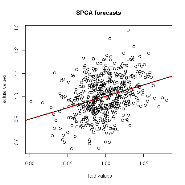

This work is licensed under a Creative Commons Attribution-NonCommercial-ShareAlike 2.5 License.
Vincent Zoonekynd
<zoonek@math.jussieu.fr>
latest modification on Sat Jan 6 10:28:22 GMT 2007