
Polynomials: curvilinear regression
Non linear regression
Local regressions
Variants of the Least Squares Method
Penalized regression
TODO: Introduction
Let us go back to our car stoping distance example: the recollections you may have from physics courses suggest that the distance could linearly depend on the square of the speed -- in other words, that it be a degree-2 polynomial in the speed.
y <- cars$dist
x <- cars$speed
o = order(x)
plot( y~x )
do.it <- function (model, col) {
  r <- lm( model )
  yp <- predict(r)
  lines( yp[o] ~ x[o], col=col, lwd=3 )
}
do.it(y~x, col="red")
do.it(y~x+I(x^2), col="blue")
do.it(y~-1+I(x^2), col="green")
legend(par("usr")[1], par("usr")[4],
       c("affine function", "degree-2 polynomial", "degree 2 monomial"),
       lwd=3,
       col=c("red", "blue", "green"),
      )
When you define a model with such a formula, the "^" character has a precise meaning; for instance, (a+b+c)^2 means a+b+c+a:b+a:c+b:c. If you add I(...), it is not interpreted and remains a square. Likewise, the "+" and "*" characters have a meaning of their own.
If you want to get rid of the intercept (it is usually a bad idea: it can encompass the effect of potentially missing variables (variables that influence the result but that have not been measured)), you can add "-1" to the formula.
We gave an example with monomials, but any function will do.
n <- 100
x <- runif(n,min=-4,max=4) + sign(x)*.2
y <- 1/x + rnorm(n)
plot(y~x)
lm( 1/y ~ x )

n <- 100
x <- rlnorm(n)^3.14
y <- x^-.1 * rlnorm(n)
plot(y~x)
lm(log(y) ~ log(x))
Actually, this is equivalent to transforming the variables.
To perform a polynomial regression, you can proceed progressively, adding the terms one by one.
y <- cars$dist
x <- cars$speed
summary( lm(y~x) )
summary( lm(y~x+I(x^2)) )
summary( lm(y~x+I(x^2)+I(x^3)) )
summary( lm(y~x+I(x^2)+I(x^3)+I(x^4)) )
summary( lm(y~x+I(x^2)+I(x^3)+I(x^4)+I(x^5)) )
Here are a few chunks of the result.
lm(formula = y ~ x)
            Estimate Std. Error t value Pr(>|t|)
(Intercept) -17.5791     6.7584  -2.601   0.0123 *
x             3.9324     0.4155   9.464 1.49e-12 ***

lm(formula = y ~ x + I(x^2))
            Estimate Std. Error t value Pr(>|t|)
(Intercept)  2.47014   14.81716   0.167    0.868
x            0.91329    2.03422   0.449    0.656
I(x^2)       0.09996    0.06597   1.515    0.136

lm(formula = y ~ x + I(x^2) + I(x^3))
             Estimate Std. Error t value Pr(>|t|)
(Intercept) -19.50505   28.40530  -0.687    0.496
x             6.80111    6.80113   1.000    0.323
I(x^2)       -0.34966    0.49988  -0.699    0.488
I(x^3)        0.01025    0.01130   0.907    0.369

lm(formula = y ~ x + I(x^2) + I(x^3) + I(x^4))
Coefficients:
              Estimate Std. Error t value Pr(>|t|)
(Intercept)  45.845412  60.849115   0.753    0.455
x           -18.962244  22.296088  -0.850    0.400
I(x^2)        2.892190   2.719103   1.064    0.293
I(x^3)       -0.151951   0.134225  -1.132    0.264
I(x^4)        0.002799   0.002308   1.213    0.232

lm(formula = y ~ x + I(x^2) + I(x^3) + I(x^4) + I(x^5))
Coefficients:
              Estimate Std. Error t value Pr(>|t|)
(Intercept) -2.650e+00  1.401e+02  -0.019    0.985
x            5.484e+00  6.736e+01   0.081    0.935
I(x^2)      -1.426e+00  1.155e+01  -0.124    0.902
I(x^3)       1.940e-01  9.087e-01   0.214    0.832
I(x^4)      -1.004e-02  3.342e-02  -0.300    0.765
I(x^5)       1.790e-04  4.648e-04   0.385    0.702
You can use the results in both directions: either you start with a simple model and you terms intil their effect becomes non-significant, or you start with a complicated model and remove the terms until the highest-degree monomial has a significant effect.
In this example, in both cases, we get a linear model (but we know, from the physics that rule the phenomenon, that is is a degree-2 polynomial).
However, the coefficients that are significantly non-zero at the begining are no longer so at the end. Even worse, at the end, there is no significant term and the p-value of the terms we want to keep is the highest!
Hopefully, we can alter this procedure so that the coefficients do not influence each other by choosing a basis other that 1, x, x^2, x^3, etc. -- an orthonormal basis.
y <- cars$dist
x <- cars$speed
summary( lm(y~poly(x,1)) )
summary( lm(y~poly(x,2)) )
summary( lm(y~poly(x,3)) )
summary( lm(y~poly(x,4)) )
summary( lm(y~poly(x,5)) )
The results are clearer: the p-values hardly change.
lm(formula = y ~ poly(x, 1))
Coefficients:
            Estimate Std. Error t value Pr(>|t|)
(Intercept)   42.980      2.175  19.761  < 2e-16 ***
poly(x, 1)   145.552     15.380   9.464 1.49e-12 ***

lm(formula = y ~ poly(x, 2))
Coefficients:
            Estimate Std. Error t value Pr(>|t|)
(Intercept)   42.980      2.146  20.026  < 2e-16 ***
poly(x, 2)1  145.552     15.176   9.591 1.21e-12 ***
poly(x, 2)2   22.996     15.176   1.515    0.136

lm(formula = y ~ poly(x, 3))
Coefficients:
            Estimate Std. Error t value Pr(>|t|)
(Intercept)    42.98       2.15  19.988  < 2e-16 ***
poly(x, 3)1   145.55      15.21   9.573  1.6e-12 ***
poly(x, 3)2    23.00      15.21   1.512    0.137
poly(x, 3)3    13.80      15.21   0.907    0.369

lm(formula = y ~ poly(x, 4))
Coefficients:
            Estimate Std. Error t value Pr(>|t|)
(Intercept)   42.980      2.139  20.090  < 2e-16 ***
poly(x, 4)1  145.552     15.127   9.622 1.72e-12 ***
poly(x, 4)2   22.996     15.127   1.520    0.135
poly(x, 4)3   13.797     15.127   0.912    0.367
poly(x, 4)4   18.345     15.127   1.213    0.232

lm(formula = y ~ poly(x, 5))
Coefficients:
            Estimate Std. Error t value Pr(>|t|)
(Intercept)   42.980      2.160  19.899  < 2e-16 ***
poly(x, 5)1  145.552     15.273   9.530 2.88e-12 ***
poly(x, 5)2   22.996     15.273   1.506    0.139
poly(x, 5)3   13.797     15.273   0.903    0.371
poly(x, 5)4   18.345     15.273   1.201    0.236
poly(x, 5)5    5.881     15.273   0.385    0.702
We can plot the evolution of those p-values.
n <- 5
p <- matrix( nrow=n, ncol=n+1 )
for (i in 1:n) {
  p[i,1:(i+1)] <- summary(lm( y ~ poly(x,i) ))$coefficients[,4]
}
matplot(p, type='l', lty=1, lwd=3)
legend( par("usr")[1], par("usr")[4],
        as.character(1:n),
        lwd=3, lty=1, col=1:n
      )
title(main="Evolution of the p-values (orthonormal polynomials)")
p <- matrix( nrow=n, ncol=n+1 )
p[1,1:2] <- summary(lm(y ~ x) )$coefficients[,4]
p[2,1:3] <- summary(lm(y ~ x+I(x^2)) )$coefficients[,4]
p[3,1:4] <- summary(lm(y ~ x+I(x^2)+I(x^3)) )$coefficients[,4]
p[4,1:5] <- summary(lm(y ~ x+I(x^2)+I(x^3)+I(x^4)) )$coefficients[,4]
p[5,1:6] <- summary(lm(y ~ x+I(x^2)+I(x^3)+I(x^4)+I(x^5)) )$coefficients[,4]
matplot(p, type='l', lty=1, lwd=3)
legend( par("usr")[1], par("usr")[4],
        as.character(1:n),
        lwd=3, lty=1, col=1:n
      )
title(main="Evolution of the p-values (non orthonormal polynomials)")
You can build this polynomial basis yourself, by hand, by starting with the family (1,x,x^2,...) and by orthonormalizing it (here, you should not see it as a polynomial, but as the predictive variable: it is a vector of dimension n; x^2 is the vector obtained by squaring its components; the family 1,x,x^2,... is a family of vectors in R^n, which we orthonormalize).
# The matrix
n <- 5
m <- matrix( ncol=n+1, nrow=length(x) )
for (i in 2:(n+1)) {
  m[,i] <- x^(i-1)
}
m[,1] <- 1
# Orthonormalization (Gram--Schmidt)
for (i in 1:(n+1)) {
  if(i==1) m[,1] <- m[,1] / sqrt( t(m[,1]) %*% m[,1] )
  else {
    for (j in 1:(i-1)) {
      m[,i] <- m[,i] - (t(m[,i]) %*% m[,j])*m[,j]
    }
    m[,i] <- m[,i] / sqrt( t(m[,i]) %*% m[,i] )
  }
}
p <- matrix( nrow=n, ncol=n+1 )
p[1,1:2] <- summary(lm(y~ -1 +m[,1:2] ))$coefficients[,4]
p[2,1:3] <- summary(lm(y~ -1 +m[,1:3] ))$coefficients[,4]
p[3,1:4] <- summary(lm(y~ -1 +m[,1:4] ))$coefficients[,4]
p[4,1:5] <- summary(lm(y~ -1 +m[,1:5] ))$coefficients[,4]
p[5,1:6] <- summary(lm(y~ -1 +m[,1:6] ))$coefficients[,4]
matplot(p, type='l', lty=1, lwd=3)
legend( par("usr")[1], par("usr")[4],
        as.character(1:n),
        lwd=3, lty=1, col=1:n
      )
title(main="Idem, orthonormalisation by hand")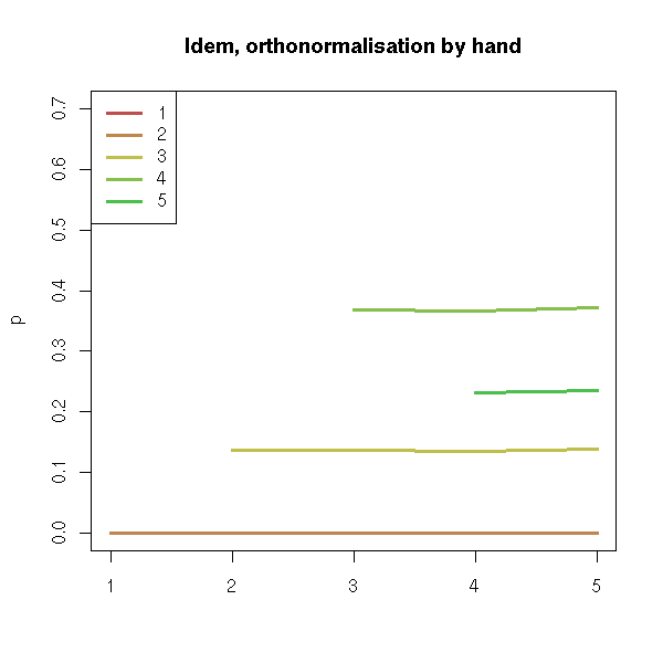
Actually, we are tackling the multilinearity problem (we will mention it agian shortly, with 1,x1,x2,x3... instead of 1,x,x^2,x^3...): by orthonormalizing the variables, we get rid of it.
Other example.
library(ts)
data(beavers)
y <- beaver1$temp
x <- 1:length(y)
plot(y~x)
for (i in 1:10) {
  r <- lm( y ~ poly(x,i) )
  lines( predict(r), type="l", col=i )
}
summary(r)
We get
>   summary(r)

             Estimate Std. Error  t value Pr(>|t|)
(Intercept)  36.86219    0.01175 3136.242  < 2e-16 ***
poly(x, i)1   0.86281    0.12549    6.875 4.89e-10 ***
poly(x, i)2  -0.73767    0.12549   -5.878 5.16e-08 ***
poly(x, i)3  -0.09652    0.12549   -0.769  0.44360
poly(x, i)4  -0.20405    0.12549   -1.626  0.10700
poly(x, i)5   1.00687    0.12549    8.023 1.73e-12 ***
poly(x, i)6   0.07253    0.12549    0.578  0.56457
poly(x, i)7   0.19180    0.12549    1.528  0.12950
poly(x, i)8   0.06011    0.12549    0.479  0.63294
poly(x, i)9  -0.22394    0.12549   -1.784  0.07730 .
poly(x, i)10 -0.39531    0.12549   -3.150  0.00214 **
---
Signif. codes:  0 `***' 0.001 `**' 0.01 `*' 0.05 `.' 0.1 ` ' 1

Residual standard error: 0.1255 on 103 degrees of freedom
Multiple R-Squared: 0.6163,     Adjusted R-squared: 0.579
F-statistic: 16.54 on 10 and 103 DF,  p-value: < 2.2e-16
Note, however, that not all relations are polynomial. (The following example is not realistic: when facing it you would first try to transform the data so that ot looks normal, and that would also solve the non-linearity problem).
> n <- 100; x <- rnorm(n); y <- exp(x); summary(lm(y~poly(x,20)))

Call:
lm(formula = y ~ poly(x, 20))

Residuals:
       Min         1Q     Median         3Q        Max
-4.803e-16 -9.921e-17 -3.675e-19  4.924e-17  1.395e-15

Coefficients:
               Estimate Std. Error   t value Pr(>|t|)
(Intercept)   1.562e+00  2.250e-17 6.943e+16  < 2e-16 ***
poly(x, 20)1  1.681e+01  2.250e-16 7.474e+16  < 2e-16 ***
poly(x, 20)2  1.174e+01  2.250e-16 5.219e+16  < 2e-16 ***
poly(x, 20)3  5.491e+00  2.250e-16 2.441e+16  < 2e-16 ***
poly(x, 20)4  1.692e+00  2.250e-16 7.522e+15  < 2e-16 ***
poly(x, 20)5  4.128e-01  2.250e-16 1.835e+15  < 2e-16 ***
poly(x, 20)6  8.163e-02  2.250e-16 3.628e+14  < 2e-16 ***
poly(x, 20)7  1.495e-02  2.250e-16 6.645e+13  < 2e-16 ***
poly(x, 20)8  2.499e-03  2.250e-16 1.111e+13  < 2e-16 ***
poly(x, 20)9  3.358e-04  2.250e-16 1.493e+12  < 2e-16 ***
poly(x, 20)10 3.825e-05  2.250e-16 1.700e+11  < 2e-16 ***
poly(x, 20)11 3.934e-06  2.250e-16 1.749e+10  < 2e-16 ***
poly(x, 20)12 3.454e-07  2.250e-16 1.536e+09  < 2e-16 ***
poly(x, 20)13 2.893e-08  2.250e-16 1.286e+08  < 2e-16 ***
poly(x, 20)14 2.235e-09  2.250e-16 9.933e+06  < 2e-16 ***
poly(x, 20)15 1.524e-10  2.250e-16 6.773e+05  < 2e-16 ***
poly(x, 20)16 1.098e-11  2.250e-16 4.883e+04  < 2e-16 ***
poly(x, 20)17 6.431e-13  2.250e-16 2.858e+03  < 2e-16 ***
poly(x, 20)18 3.628e-14  2.250e-16 1.613e+02  < 2e-16 ***
poly(x, 20)19 1.700e-15  2.250e-16 7.558e+00  6.3e-11 ***
poly(x, 20)20 5.790e-16  2.250e-16 2.574e+00   0.0119 *
---
Signif. codes:  0 `***' 0.001 `**' 0.01 `*' 0.05 `.' 0.1 ` ' 1

Residual standard error: 2.25e-16 on 79 degrees of freedom
Multiple R-Squared:     1,      Adjusted R-squared:     1
F-statistic: 4.483e+32 on 20 and 79 DF,  p-value: < 2.2e-16

n <- 100
x <- rnorm(n)
y <- exp(x)
plot(y~x)
title(main="Non-polynomial relation")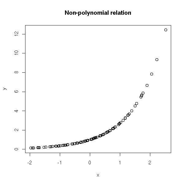
If you add some noise:
> n <- 100; x <- rnorm(n); y <- exp(x) + .1*rnorm(n); summary(lm(y~poly(x,20)))

Call:
lm(formula = y ~ poly(x, 20))

Residuals:
       Min         1Q     Median         3Q        Max
-2.059e-01 -5.577e-02 -4.859e-05  5.322e-02  3.271e-01

Coefficients:
               Estimate Std. Error t value Pr(>|t|)
(Intercept)    1.617035   0.010222 158.185   <2e-16 ***
poly(x, 20)1  15.802708   0.102224 154.588   <2e-16 ***
poly(x, 20)2  11.282604   0.102224 110.371   <2e-16 ***
poly(x, 20)3   4.688413   0.102224  45.864   <2e-16 ***
poly(x, 20)4   1.433877   0.102224  14.027   <2e-16 ***
poly(x, 20)5   0.241665   0.102224   2.364   0.0205 *
poly(x, 20)6  -0.009086   0.102224  -0.089   0.9294
poly(x, 20)7  -0.097021   0.102224  -0.949   0.3455
poly(x, 20)8   0.133978   0.102224   1.311   0.1938
poly(x, 20)9   0.077034   0.102224   0.754   0.4533
poly(x, 20)10  0.200996   0.102224   1.966   0.0528 .
poly(x, 20)11 -0.168632   0.102224  -1.650   0.1030
poly(x, 20)12  0.161890   0.102224   1.584   0.1173
poly(x, 20)13 -0.049974   0.102224  -0.489   0.6263
poly(x, 20)14  0.090020   0.102224   0.881   0.3812
poly(x, 20)15 -0.228817   0.102224  -2.238   0.0280 *
poly(x, 20)16 -0.005180   0.102224  -0.051   0.9597
poly(x, 20)17 -0.015934   0.102224  -0.156   0.8765
poly(x, 20)18  0.053635   0.102224   0.525   0.6013
poly(x, 20)19  0.059976   0.102224   0.587   0.5591
poly(x, 20)20  0.226613   0.102224   2.217   0.0295 *
---
Signif. codes:  0 `***' 0.001 `**' 0.01 `*' 0.05 `.' 0.1 ` ' 1

Residual standard error: 0.1022 on 79 degrees of freedom
Multiple R-Squared: 0.9979,     Adjusted R-squared: 0.9974
F-statistic:  1920 on 20 and 79 DF,  p-value: < 2.2e-16

n <- 100
x <- rnorm(n)
y <- exp(x) + .1*rnorm(n)
plot(y~x)
title(main="Non-polynomial relation")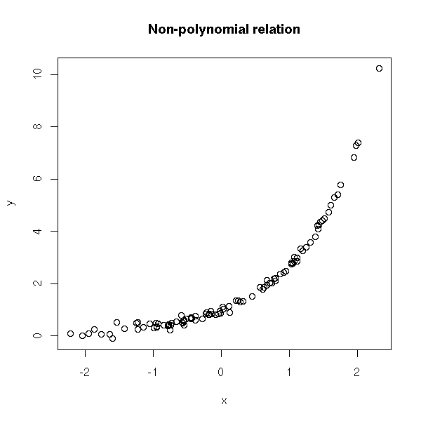
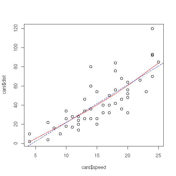
The broken line regression is local (what happens for a given value of X does not depend on what happens for very different values of X), but not smooth. On the contrary, polynomial regression is smooth but not local. Spline regression provides a local and smooth regression.
Splines should be used (at least) when looking for a model: they allow you to see, graphically, if a non-linear model is a good idea and, if not, gives some insight on the shape of that model.
library(modreg)
plot(cars$speed, cars$dist)
lines( smooth.spline(cars$speed, cars$dist), col='red')
abline(lm(dist~speed,data=cars), col='blue', lty=2)
plot(quakes$long, quakes$lat)
lines( smooth.spline(quakes$long, quakes$lat), col='red', lwd=3)
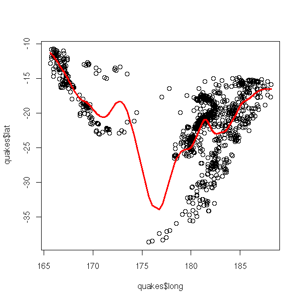
There are several kinds of splines: cubic splines (of class C^2, obtained by glueing degree-3 polynomials), that we have just used, or restricted cubic splines (idem but the polynomials at both end of the interval are affine -- otherwise, extrapolating outside the interval would not yield reliable results), obtained by the "rcs" function in the "Design" package.
library(Design)
# 4-node spline
r3 <- lm( quakes$lat ~ rcs(quakes$long) )
plot( quakes$lat ~ quakes$long )
o <- order(quakes$long)
lines( quakes$long[o], predict(r)[o], col='red', lwd=3 )
r <- lm( quakes$lat ~ rcs(quakes$long,10) )
lines( quakes$long[o], predict(r)[o], col='blue', lwd=6, lty=3 )
title(main="Regression with rcs")
legend( par("usr")[1], par("usr")[3], yjust=0,
        c("4 knots", "10 knots"),
        lwd=c(3,3), lty=c(1,3), col=c("red", "blue") )
There are also a few functions in the "splines" package: "bs" for splines and "ns" for restricted splines.
library(splines)
data(quakes)
x <- quakes[,2]
y <- quakes[,1]
o <- order(x)
x <- x[o]
y <- y[o]
r1 <- lm( y ~ bs(x,df=10) )
r2 <- lm( y ~ ns(x,df=6) )
plot(y~x)
lines(predict(r1)~x, col='red', lwd=3)
lines(predict(r2)~x, col='green', lwd=3)
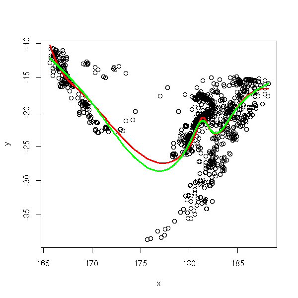
TODO
?SafePrediction
# The manual asks us to be cautious with predictions
# for ither values of x: I do not see any problem.
plot(y~x)
xp <- seq(min(x), max(x), length=200)
lines(predict(r2) ~ x, col='green', lwd=3)
lines(xp, predict(r2,data.frame(x=xp)), col='blue', lwd=7, lty=3)
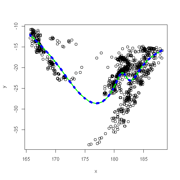
TODO: wavelets
The data can suggest a regression in a certain basis. Thus, in higher dimensions, you can try to write Y as a sum of gaussians: you will use various heuristics to find the number, the center and the variance of those gaussians (this is not linear at all), then, you would use least squares to find the coefficients.
TODO: example
You can also consider really non-linear models (the preceding polynomial regressions were linear: the polynomials were considered as a linear combination of monomials -- in the end, it was always a linear regression). You should only use them with a valid reason, e.g., a well-established physical model of the phenomenon -- this is often the case in chemistry -- more generally, when you know that there should be asymptotes somewhere.
Here are a few examples.
Expenential growth or decrease, Y = a e^(bX) + noise
n <- 100
x <- seq(-2,2,length=n)
y <- exp(x)
plot(y~x, type='l', lwd=3)
title(main='Expenential growth')

x <- seq(-2,2,length=n)
y <- exp(-x)
plot(y~x, type='l', lwd=3)
title(main='Exponential Decrease')
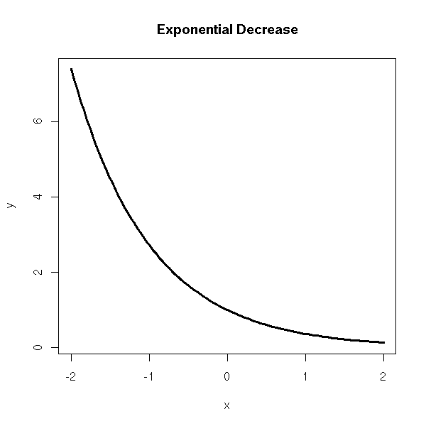
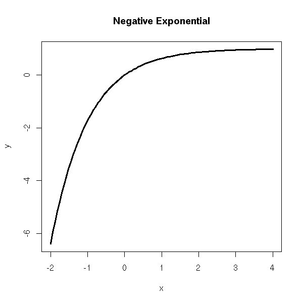
Negative exponential, Y = a(1-e^(bX)) + noise
x <- seq(-2,4,length=n)
y <- 1-exp(-x)
plot(y~x, type='l', lwd=3)
title(main='Negative Exponential')
Double exponential, Y = u/(u-v) * (e^(-vX) - e^(-uX)) + noise
x <- seq(0,5,length=n)
u <- 1
v <- 2
y <- u/(u-v) * (exp(-v*x) - exp(-u*x))
plot(y~x, type='l', lwd=3)
title(main='Double Exponential')

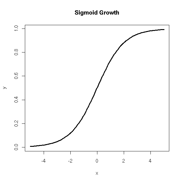
Sigmoid growth ("sigmoid" means "S-shaped"), Y = a/( 1+ce^(-bX) ) + noise
x <- seq(-5,5,length=n)
y <- 1/(1+exp(-x))
plot(y~x, type='l', lwd=3)
title(main='Sigmoid Growth')
Less symetric sigmoid, Y = a exp( -ce^(-bX) ) + noise
x <- seq(-2,5,length=n)
y <- exp(-exp(-x))
plot(y~x, type='l', lwd=3)
title(main='Less Symetric Sigmoid')

To perform those regressions, you can still use the Least Squares (LS) method, but you get a non-linear system: you can solve it with numeric methods, such as the Newton-Raphson.
library(help=nls)
library(nls)
?nls
You define an f(x,p) function, where x is the variable and p a vector containing the parameters. You will use it as f(x,c(a,b,c)). You HAVE to provide initial estimates (guesses) of the paramters. They need not be too precise, but they should not be too far away from minimum of the function to minimize: otherwise, the algorithm could diverge, take a long time to converge, or (more likely) converge to a local minimum...
library(nls)
f <- function (x,p) {
  u <- p[1]
  v <- p[2]
  u/(u-v) * (exp(-v*x) - exp(-u*x))
}
n <- 100
x <- runif(n,0,2)
y <- f(x, c(3.14,2.71)) + .1*rnorm(n)
r <- nls( y ~ f(x,c(a,b)), start=c(a=3, b=2.5) )
plot(y~x)
xx <- seq(0,2,length=200)
lines(xx, f(xx,r$m$getAllPars()), col='red', lwd=3)
lines(xx, f(xx,c(3.14,2.71)), lty=2)
Here is the result.
> summary(r)
Formula: y ~ f(x, c(a, b))

Parameters:
  Estimate Std. Error t value Pr(>|t|)
a   3.0477     0.3358   9.075 1.23e-14 ***
b   2.6177     0.1459  17.944  < 2e-16 ***
---
Signif. codes:  0 `***' 0.001 `**' 0.01 `*' 0.05 `.' 0.1 ` ' 1

Residual standard error: 0.1059 on 98 degrees of freedom

Correlation of Parameter Estimates:
         a
b -0.06946
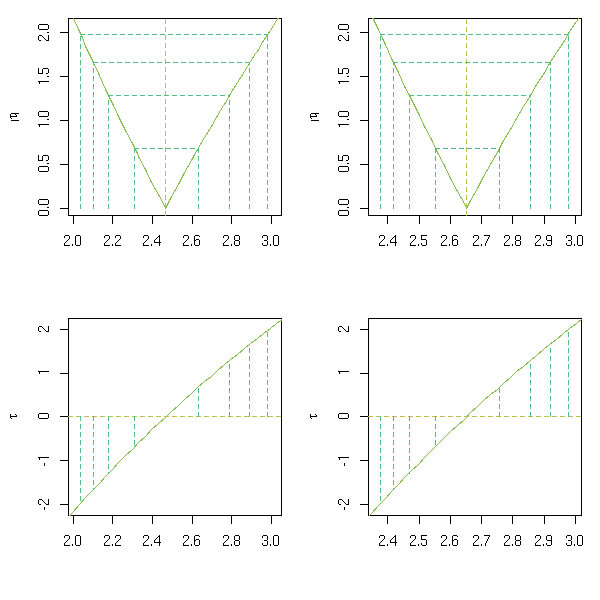
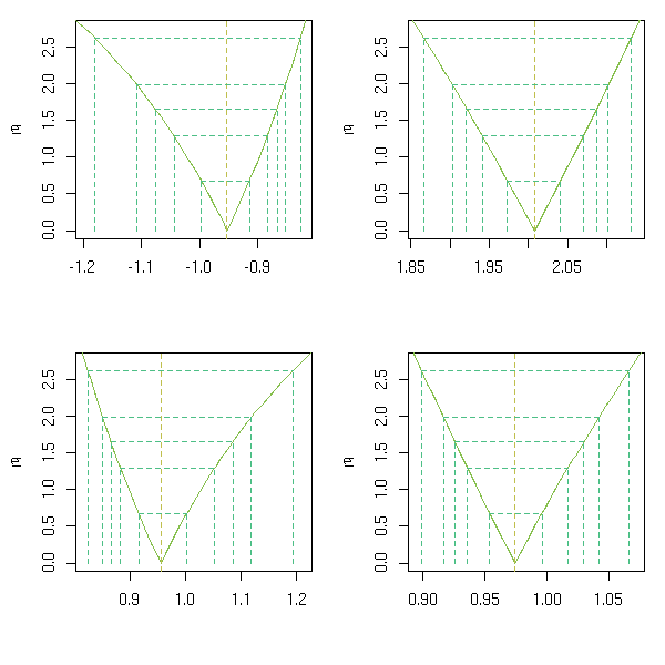
You can plot the confidence intervals.
op <- par(mfrow=c(2,2))
p <- profile(r)
plot(p, conf = c(95, 90, 80, 50)/100)
plot(p, conf = c(95, 90, 80, 50)/100, absVal = FALSE)
par(op)
There are a few predefined non-linear models. For some of the, R can find good starting values for the parameters.
rm(r)
while(!exists("r")) {
  x <- runif(n,0,2)
  y <- SSbiexp(x,1,1,-1,2) + .01*rnorm(n)
  try(  r <- nls(y ~ SSbiexp(x,a,u,b,v))  )
}
plot(y~x)
xx <- seq(0,2,length=200)
lines(xx, SSbiexp(xx,
                  r$m$getAllPars()[1],
                  r$m$getAllPars()[2],
                  r$m$getAllPars()[3],
                  r$m$getAllPars()[4]
                  ), col='red', lwd=3)
title(main='biexponential')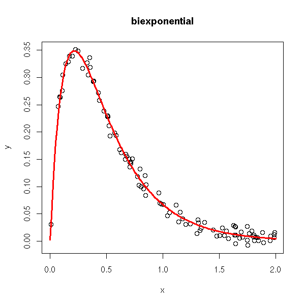
op <- par(mfrow=c(2,2))
try(plot(profile(r)))
par(op)
rm(r)
while(!exists("r")) {
  x <- runif(n,-5,5)
  y <- SSlogis(x,1,0,1) + .1*rnorm(n)
  try( r <- nls(y ~ SSlogis(x,a,m,s)) )
}
plot(y~x)
xx <- seq(-5,5,length=200)
lines(xx, SSlogis(xx,
                  r$m$getAllPars()[1],
                  r$m$getAllPars()[2],
                  r$m$getAllPars()[3]
                  ), col='red', lwd=3)
title(main='logistic')
rm(r)
while(!exists("r")) {
  x <- runif(n,-5,5)
  y <- SSfpl(x,-1,1,0,1) + .1*rnorm(n)
  try( r <- nls(y ~ SSfpl(x,a,b,m,s)) )
}
plot(y~x)
xx <- seq(-5,5,length=200)
lines(xx, SSfpl(xx,
                  r$m$getAllPars()[1],
                  r$m$getAllPars()[2],
                  r$m$getAllPars()[3],
                  r$m$getAllPars()[4]
                  ), col='red', lwd=3)
title(main='4-parameter logistic model')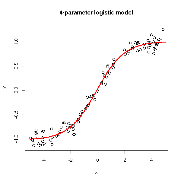
rm(r)
while(!exists("r")) {
  x <- runif(n,-5,5)
  y <- SSmicmen(x,1,1) + .01*rnorm(n)
  try( r <- nls(y ~ SSmicmen(x,m,h)) )
}
plot(y~x, ylim=c(-5,5))
xx <- seq(-5,5,length=200)
lines(xx, SSmicmen(xx,
                  r$m$getAllPars()[1],
                  r$m$getAllPars()[2]
                  ), col='red', lwd=3)
title(main='Michaelis-Menten')
rm(r)
while(!exists("r")) {
  x <- runif(n,0,5)
  y <- SSmicmen(x,1,1) + .1*rnorm(n)
  try( r <- nls(y ~ SSmicmen(x,m,h)) )
}
plot(y~x)
xx <- seq(0,5,length=200)
lines(xx, SSmicmen(xx,
                  r$m$getAllPars()[1],
                  r$m$getAllPars()[2]
                  ), col='red', lwd=3)
title(main='Michaelis-Menten')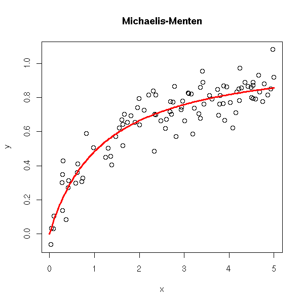
rm(r)
while(!exists("r")) {
  x <- runif(n,0,1)
  y <- SSfol(1,x,1,2,1) + .1*rnorm(n)
  try( r <- nls(y ~ SSfol(1,x,a,b,c)) )
}
plot(y~x)
xx <- seq(0,1,length=200)
lines(xx, SSfol(1,
                   xx,
                   r$m$getAllPars()[1],
                   r$m$getAllPars()[2],
                   r$m$getAllPars()[3]
                  ), col='red', lwd=3)
title(main='SSfol')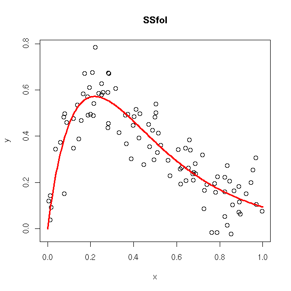
rm(r)
while(!exists("r")) {
  x <- runif(n,0,2)
  y <- SSasymp(x,1,.5,1) + .1*rnorm(n)
  try( r <- nls(y ~ SSasymp(x,a,b,c)) )
}
plot(y~x, xlim=c(-.5,2),ylim=c(0,1.3))
xx <- seq(-1,2,length=200)
lines(xx, SSasymp(xx,
                  r$m$getAllPars()[1],
                  r$m$getAllPars()[2],
                  r$m$getAllPars()[3]
                 ), col='red', lwd=3)
title(main='SSasymp')
# See also SSasympOff et SSasympOrig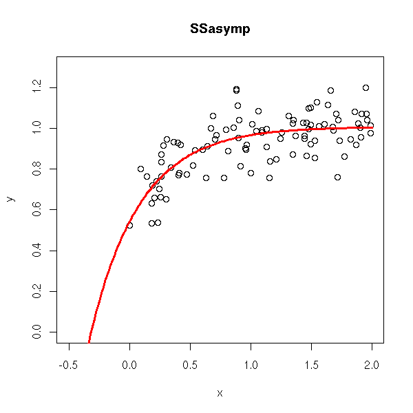
The manual explains how to interpret those parameters.
# Copied from the manual
xx <- seq(0, 5, len = 101)
yy <- 5 - 4 * exp(-xx/(2*log(2)))
par(mar = c(0, 0, 4.1, 0))
plot(xx, yy, type = "l", axes = FALSE, ylim = c(0,6), xlim = c(-1, 5),
     xlab = "", ylab = "", lwd = 2,
     main = "Parameters in the SSasymp model")
usr <- par("usr")
arrows(usr[1], 0, usr[2], 0, length = 0.1, angle = 25)
arrows(0, usr[3], 0, usr[4], length = 0.1, angle = 25)
text(usr[2] - 0.2, 0.1, "x", adj = c(1, 0))
text(-0.1, usr[4], "y", adj = c(1, 1))
abline(h = 5, lty = 2, lwd = 0)
arrows(-0.8, 2.1, -0.8, 0, length = 0.1, angle = 25)
arrows(-0.8, 2.9, -0.8, 5, length = 0.1, angle = 25)
text(-0.8, 2.5, expression(phi[1]), adj = c(0.5, 0.5))
segments(-0.4, 1, 0, 1, lty = 2, lwd = 0.75)
arrows(-0.3, 0.25, -0.3, 0, length = 0.07, angle = 25)
arrows(-0.3, 0.75, -0.3, 1, length = 0.07, angle = 25)
text(-0.3, 0.5, expression(phi[2]), adj = c(0.5, 0.5))
segments(1, 3.025, 1, 4, lty = 2, lwd = 0.75)
arrows(0.2, 3.5, 0, 3.5, length = 0.08, angle = 25)
arrows(0.8, 3.5, 1, 3.5, length = 0.08, angle = 25)
text(0.5, 3.5, expression(t[0.5]), adj = c(0.5, 0.5))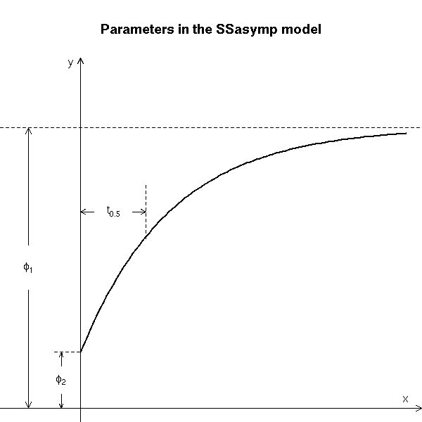
# Copied from the manual
xx <- seq(0.5, 5, len = 101)
yy <- 5 * (1 -  exp(-(xx - 0.5)/(2*log(2))))
par(mar = c(0, 0, 4.0, 0))
plot(xx, yy, type = "l", axes = FALSE, ylim = c(0,6), xlim = c(-1, 5),
     xlab = "", ylab = "", lwd = 2,
     main = "Parameters in the SSasympOff model")
usr <- par("usr")
arrows(usr[1], 0, usr[2], 0, length = 0.1, angle = 25)
arrows(0, usr[3], 0, usr[4], length = 0.1, angle = 25)
text(usr[2] - 0.2, 0.1, "x", adj = c(1, 0))
text(-0.1, usr[4], "y", adj = c(1, 1))
abline(h = 5, lty = 2, lwd = 0)
arrows(-0.8, 2.1, -0.8, 0, length = 0.1, angle = 25)
arrows(-0.8, 2.9, -0.8, 5, length = 0.1, angle = 25)
text(-0.8, 2.5, expression(phi[1]), adj = c(0.5, 0.5))
segments(0.5, 0, 0.5, 3, lty = 2, lwd = 0.75)
text(0.5, 3.1, expression(phi[3]), adj = c(0.5, 0))
segments(1.5, 2.525, 1.5, 3, lty = 2, lwd = 0.75)
arrows(0.7, 2.65, 0.5, 2.65, length = 0.08, angle = 25)
arrows(1.3, 2.65, 1.5, 2.65, length = 0.08, angle = 25)
text(1.0, 2.65, expression(t[0.5]), adj = c(0.5, 0.5))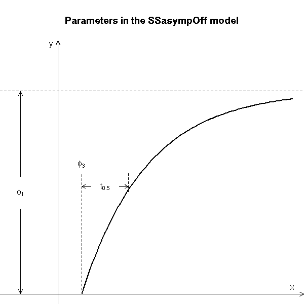
# Copied from the manual
xx <- seq(0, 5, len = 101)
yy <- 5 * (1- exp(-xx/(2*log(2))))
par(mar = c(0, 0, 3.5, 0))
plot(xx, yy, type = "l", axes = FALSE, ylim = c(0,6), xlim = c(-1, 5),
     xlab = "", ylab = "", lwd = 2,
     main = "Parameters in the SSasympOrig model")
usr <- par("usr")
arrows(usr[1], 0, usr[2], 0, length = 0.1, angle = 25)
arrows(0, usr[3], 0, usr[4], length = 0.1, angle = 25)
text(usr[2] - 0.2, 0.1, "x", adj = c(1, 0))
text(-0.1, usr[4], "y", adj = c(1, 1))
abline(h = 5, lty = 2, lwd = 0)
arrows(-0.8, 2.1, -0.8, 0, length = 0.1, angle = 25)
arrows(-0.8, 2.9, -0.8, 5, length = 0.1, angle = 25)
text(-0.8, 2.5, expression(phi[1]), adj = c(0.5, 0.5))
segments(1, 2.525, 1, 3.5, lty = 2, lwd = 0.75)
arrows(0.2, 3.0, 0, 3.0, length = 0.08, angle = 25)
arrows(0.8, 3.0, 1, 3.0, length = 0.08, angle = 25)
text(0.5, 3.0, expression(t[0.5]), adj = c(0.5, 0.5))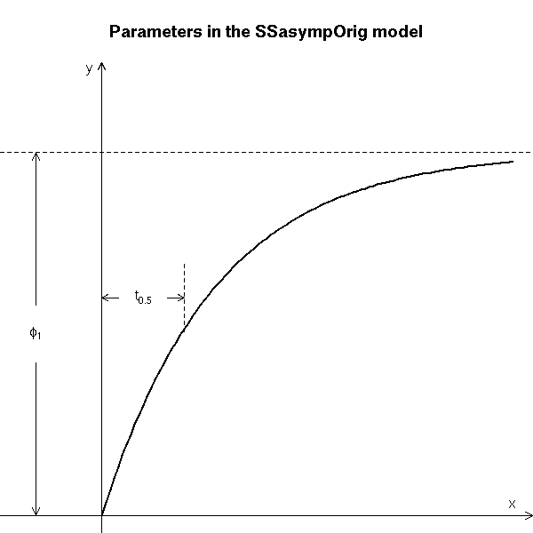
# Copied from the manual
xx <- seq(-0.5, 5, len = 101)
yy <- 1 + 4 / ( 1 + exp((2-xx)))
par(mar = c(0, 0, 3.5, 0))
plot(xx, yy, type = "l", axes = FALSE, ylim = c(0,6), xlim = c(-1, 5),
     xlab = "", ylab = "", lwd = 2,
     main = "Parameters in the SSfpl model")
usr <- par("usr")
arrows(usr[1], 0, usr[2], 0, length = 0.1, angle = 25)
arrows(0, usr[3], 0, usr[4], length = 0.1, angle = 25)
text(usr[2] - 0.2, 0.1, "x", adj = c(1, 0))
text(-0.1, usr[4], "y", adj = c(1, 1))
abline(h = 5, lty = 2, lwd = 0)
arrows(-0.8, 2.1, -0.8, 0, length = 0.1, angle = 25)
arrows(-0.8, 2.9, -0.8, 5, length = 0.1, angle = 25)
text(-0.8, 2.5, expression(phi[1]), adj = c(0.5, 0.5))
abline(h = 1, lty = 2, lwd = 0)
arrows(-0.3, 0.25, -0.3, 0, length = 0.07, angle = 25)
arrows(-0.3, 0.75, -0.3, 1, length = 0.07, angle = 25)
text(-0.3, 0.5, expression(phi[2]), adj = c(0.5, 0.5))
segments(2, 0, 2, 3.3, lty = 2, lwd = 0.75)
text(2, 3.3, expression(phi[3]), adj = c(0.5, 0))
segments(3, 1+4/(1+exp(-1)) - 0.025, 3, 2.5, lty = 2, lwd = 0.75)
arrows(2.3, 2.7, 2.0, 2.7, length = 0.08, angle = 25)
arrows(2.7, 2.7, 3.0, 2.7, length = 0.08, angle = 25)
text(2.5, 2.7, expression(phi[4]), adj = c(0.5, 0.5))
# Copied from the manual
xx <- seq(-0.5, 5, len = 101)
yy <- 5 / ( 1 + exp((2-xx)))
par(mar = c(0, 0, 3.5, 0))
plot(xx, yy, type = "l", axes = FALSE, ylim = c(0,6), xlim = c(-1, 5),
     xlab = "", ylab = "", lwd = 2,
     main = "Parameters in the SSlogis model")
usr <- par("usr")
arrows(usr[1], 0, usr[2], 0, length = 0.1, angle = 25)
arrows(0, usr[3], 0, usr[4], length = 0.1, angle = 25)
text(usr[2] - 0.2, 0.1, "x", adj = c(1, 0))
text(-0.1, usr[4], "y", adj = c(1, 1))
abline(h = 5, lty = 2, lwd = 0)
arrows(-0.8, 2.1, -0.8, 0, length = 0.1, angle = 25)
arrows(-0.8, 2.9, -0.8, 5, length = 0.1, angle = 25)
text(-0.8, 2.5, expression(phi[1]), adj = c(0.5, 0.5))
segments(2, 0, 2, 4.0, lty = 2, lwd = 0.75)
text(2, 4.0, expression(phi[2]), adj = c(0.5, 0))
segments(3, 5/(1+exp(-1)) + 0.025, 3, 4.0, lty = 2, lwd = 0.75)
arrows(2.3, 3.8, 2.0, 3.8, length = 0.08, angle = 25)
arrows(2.7, 3.8, 3.0, 3.8, length = 0.08, angle = 25)
text(2.5, 3.8, expression(phi[3]), adj = c(0.5, 0.5))
# Copied from the manual
xx <- seq(0, 5, len = 101)
yy <- 5 * xx/(1+xx)
par(mar = c(0, 0, 3.5, 0))
plot(xx, yy, type = "l", axes = FALSE, ylim = c(0,6), xlim = c(-1, 5),
     xlab = "", ylab = "", lwd = 2,
     main = "Parameters in the SSmicmen model")
usr <- par("usr")
arrows(usr[1], 0, usr[2], 0, length = 0.1, angle = 25)
arrows(0, usr[3], 0, usr[4], length = 0.1, angle = 25)
text(usr[2] - 0.2, 0.1, "x", adj = c(1, 0))
text(-0.1, usr[4], "y", adj = c(1, 1))
abline(h = 5, lty = 2, lwd = 0)
arrows(-0.8, 2.1, -0.8, 0, length = 0.1, angle = 25)
arrows(-0.8, 2.9, -0.8, 5, length = 0.1, angle = 25)
text(-0.8, 2.5, expression(phi[1]), adj = c(0.5, 0.5))
segments(1, 0, 1, 2.7, lty = 2, lwd = 0.75)
text(1, 2.7, expression(phi[2]), adj = c(0.5, 0))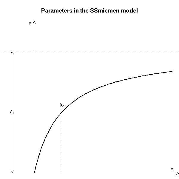
For other models, the big problem is to find good starting values of the parameters, not too far from the actual values.
x <- runif(100)
w <- runif(100)
y <- x^2.4*w^3.2+rnorm(100,0,0.01)
# Linear regression to get the initial guesses
r1 <- lm(log(y) ~ log(x)+log(w)-1)
r2 <- nls(y~x^a*w^b,start=list(a=coef(r1)[1],b=coef(r1)[2]))

> coef(r1)
  log(x)   log(w)
1.500035 2.432708
> coef(r2)
       a        b
2.377525 3.185556
When doing all those computations, I realize that those methods do not always work. Here are some sample error messages I got. (It might not be a problem with real data -- but on the contrary, it might: be careful, check that the algorithm has not crashed and that it has converged.) This is why I used the "try" command in the examples above.
> r <- nls(y ~ SSfol(1,x,a,b,c))
Error in numericDeriv(form[[3]], names(ind), env):
  Missing value or an Infinity produced when evaluating the model
In addition: Warning messages:
1: NaNs produced in: log(x)
2: NaNs produced in: log(x)

> r <- nls(y ~ SSfol(1,x,a,b,c))
Error in nls(resp ~ (Dose * (exp(-input * exp(lKe)) - exp(-input * exp(lKa))))/(exp(lKa) - :
  singular gradient

Error in nls(y ~ cbind(exp(-exp(lrc1) * x), exp(-exp(lrc2) * x)), data = xy,  :
  step factor 0.000488281 reduced below `minFactor' of 0.000976562
Comparing non-linear models is trickier. There is however an "anova.nls" function.
library(nls)
?anova.nls
TODO...
See the rnls function, in the sfsmisc package.
Did I stress the difference between parametric and non-parametric non-linear regression?
TODO: Also check the "drc" package (sometimes presented as an extension of "nls").
A very simple way of seeing wether a linear regression is a good idea (or if a more complex model is advisable) consists in putting the data into two clusters, according to the values of one of the predictive variables (say, X1<median(X1) and X1>median(X1)) and performing a linear regression on each of those two sub-samples.
broken.line <- function (x, y) {
  n <- length(x)
  n2 = floor(n/2)
  o <- order(x)
  m <- mean(c(x[o[n2+0:1]]))
  x1 <- x[o[1:n2]]
  y1 <- y[o[1:n2]]
  n2 <- n2+1
  x2 <- x[o[n2:n]]
  y2 <- y[o[n2:n]]
  r1 <- lm(y1~x1)
  r2 <- lm(y2~x2)
  plot(y~x)
  segments(x[o[1]], r1$coef[1] + x[o[1]]*r1$coef[2],
           m, r1$coef[1] + m *r1$coef[2],
           col='red')
  segments(m, r2$coef[1] + m*r2$coef[2],
           x[o[n]], r2$coef[1] + x[o[n]] *r2$coef[2],
           col='blue')
  abline(v=m, lty=3)
}
set.seed(1)
n <- 10
x <- runif(n)
y <- 1-x+.2*rnorm(n)
broken.line(x,y)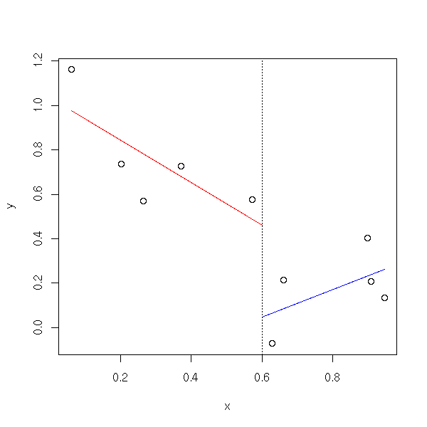
z <- x*(1-x)
broken.line(x,z)

This is not continuous: you can ask that the two segments touch each other.
broken.line <- function (x,y) {
  n <- length(x)
  o <- order(x)
  n1 <- floor((n+1)/2)
  n2 <- ceiling((n+1)/2)
  m <- mean(c( x[o[n1]], x[o[n2]] ))
  plot(y~x)
  B1 <- function (xx) {
    x <- xx
    x[xx<m] <- m - x[xx<m]
    x[xx>=m] <- 0
    x
  }
  B2 <- function (xx) {
    x <- xx
    x[xx>m] <- x[x>m] -m
    x[xx<=m] <- 0
    x
  }
  x1 <- B1(x)
  x2 <- B2(x)
  r <- lm(y~x1+x2)
  xx <- seq(x[o[1]],x[o[n]],length=100)
  yy <- predict(r, data.frame(x1=B1(xx), x2=B2(xx)))
  lines( xx, yy, col='red' )
  abline(v=m, lty=3)
}
broken.line(x,y)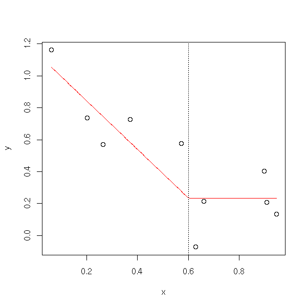
broken.line(x,z)

Exercise left to the reader: Modify the preceding function so that it uses an arbitrary number of segments (given as argument of the function).
There is already a function to perform those "broken-line regressions".
set.seed(5)
n <- 200
x <- rnorm(n)
k <- rnorm(1)
x1 <- ifelse( x < k, x - k, 0 )
x2 <- ifelse( x < k, 0, x - k )
a <- rnorm(1)
b1 <- rnorm(1)
b2 <- rnorm(1)
y <- a + b1 * x1 + b2 * x2 + .2*rnorm(n)
plot( y ~ x, col = ifelse(x < k, "blue", "green") )
abline(a - k*b1, b1, col="blue", lwd=2, lty=2)
abline(a - k*b2, b2, col="green", lwd=2, lty=2)

library(segmented)
r <- segmented( lm(y~x),
                x,        # Variable along which we are allowed to cut
                0         # Initial values of the cut-points
              )           # (there can be several)
plot(x, y)
o <- order(x)
lines( x[o], r$fitted.values[o], col="red", lwd=3 )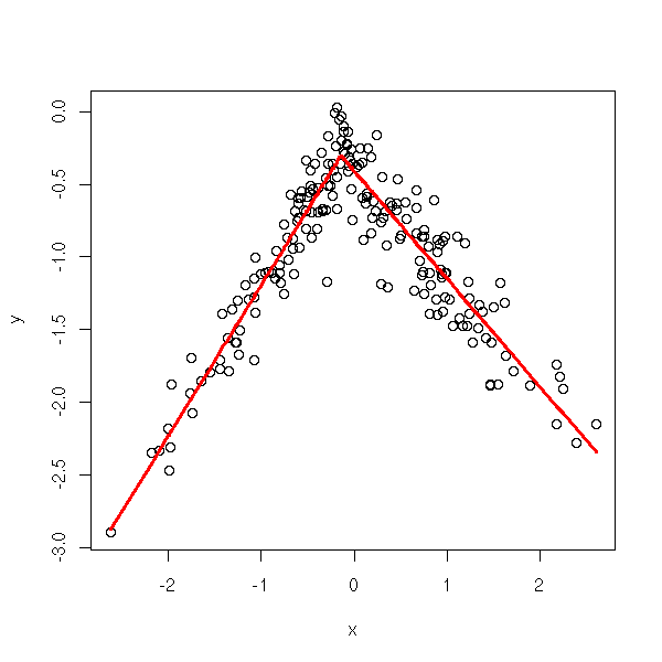
> summary( segmented( lm(y ~ x), x, psi=c(0) ) )

      ***Regression Model with Segmented Relationship(s)***

Call:
segmented.lm(obj = lm(y ~ x), Z = x, psi = c(0))

Estimated Break-Point(s):
     Est.   St.Err
-0.14370  0.02641

t value for the gap-variable(s) V:  4.173e-16

Meaningful coefficients of the linear terms:
            Estimate Std. Error t value
(Intercept)  -0.1528    0.03836  -3.983
x             1.0390    0.03788  27.431
U.x          -1.7816    0.04829 -36.896


Residual standard error: 0.202 on 196 degrees of freedom
Multiple R-Squared: 0.875,  Adjusted R-squared: 0.873

Convergence attained in 4 iterations with relative change 0
> k
[1] -0.1137
See also
library(structchange)
?breakpoints
TODO: is it a line?
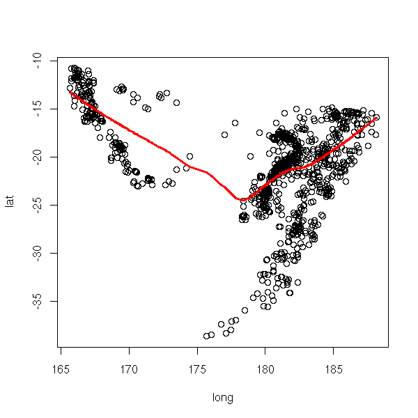
The "lowess" function yields a curve (a generalization of our previous "continuous broken line") "close" to the cloud of points.
set.seed(1)
n <- 10
x <- runif(n)
y <- 1-x+.2*rnorm(n)
z <- x*(1-x)  # Same data as above
plot(y~x)
lines(lowess(x,y), col="red")

plot(z~x)
lines(lowess(x,z), col="red")

data(quakes)
plot(lat~long, data=quakes)
lines(lowess(quakes$long, quakes$lat), col='red', lwd=3)
The "scatter.smooth" has a similar purpose.
TODO: example
Here, for each point for which we want a prediction, we compute the mean of the nearby points (if the observations are ordered, as for time series, we would the n previous points, so as not to peer into the future).
In other words, we try to locally approximate the cloud of points by a horizontal line.
n <- 1000
x <- runif(n, min=-1,max=1)
y <- (x-1)*x*(x+1) + .5*rnorm(n)
# Do not use this code for large data sets.
moyenne.mobile <- function (y,x, r=.1) {
  o <- order(x)
  n <- length(x)
  m <- floor((1-r)*n)
  p <- n-m
  x1 <- vector(mode='numeric',length=m)
  y1 <- vector(mode='numeric',length=m)
  y2 <- vector(mode='numeric',length=m)
  y3 <- vector(mode='numeric',length=m)
  for (i in 1:m) {
    xx <- x[ o[i:(i+p)] ]
    yy <- y[ o[i:(i+p)] ]
    x1[i] <- mean(xx)
    y1[i] <- quantile(yy,.25)
    y2[i] <- quantile(yy,.5)
    y3[i] <- quantile(yy,.75)
  }
  plot(y~x)
  lines(x1,y2,col='red', lwd=3)
  lines(x1,y1,col='blue', lwd=2)
  lines(x1,y3,col='blue', lwd=2)
}
moyenne.mobile(y,x)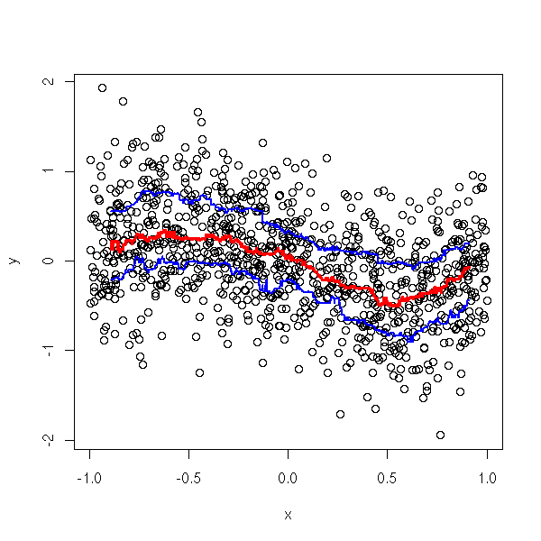
TODO: take the previous example with the "filter" command -- no loop.
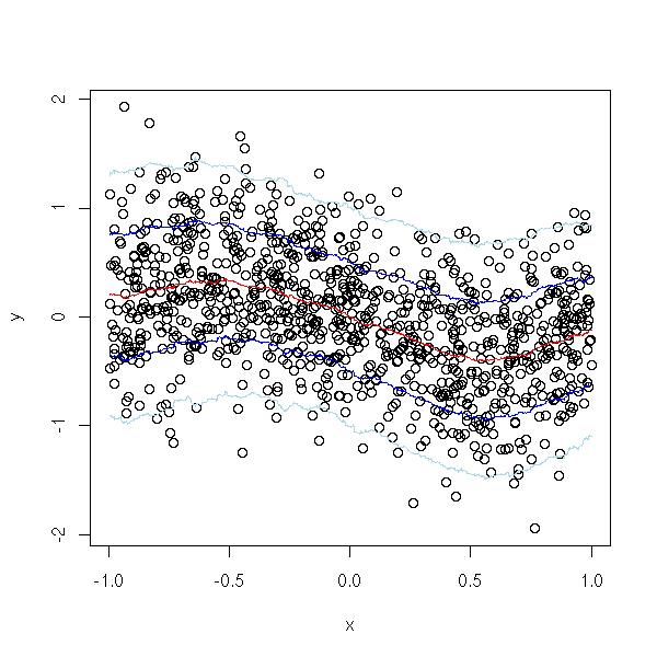
There is a similar function in the "gregmisc" bundle.
library(gregmisc)
bandplot(x,y)
TODO: give the other alternatives.
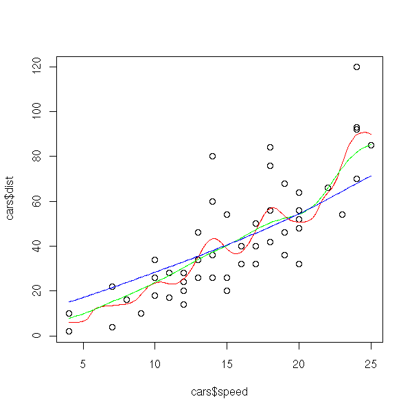
The "ksmooth" function is very similar (the observations are weighted by a kernel).
library(modreg)
plot(cars$speed, cars$dist)
lines(ksmooth(cars$speed, cars$dist, "normal", bandwidth=2), col='red')
lines(ksmooth(cars$speed, cars$dist, "normal", bandwidth=5), col='green')
lines(ksmooth(cars$speed, cars$dist, "normal", bandwidth=10), col='blue')
The method we have just presented, the Moving Average (MA), has many variants. First, we can change the kernel.
TODO: I keep on using the word "kernel": be sure to define it. (above, when I use the "filter" function to compute MAs).
curve(dnorm(x), xlim=c(-3,3), ylim=c(0,1.1))
x <- seq(-3,3,length=200)
D.Epanechikov <- function (t) {
  ifelse(abs(t)<1, 3/4*(1-t^2), 0)
}
lines(D.Epanechikov(x) ~ x, col='red')
D.tricube <- function (t) { # aka "triweight kernel"
  ifelse(abs(t)<1, (1-abs(t)^3)^3, 0)
}
lines(D.tricube(x) ~ x, col='blue')
legend( par("usr")[1], par("usr")[4], yjust=1,
        c("noyau gaussien", "noyau d'Epanechikov", "noyau tricube"),
        lwd=1, lty=1,
        col=c(par('fg'),'red', 'blue'))
title(main="Differents kernels")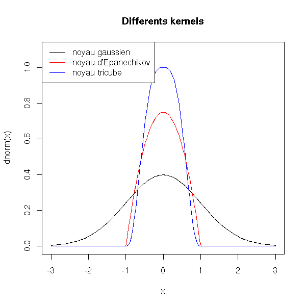
More formally, if D is one of the functions above, the smoothing procedure finds the function f that minimizes
RSS(f,x0) = Sum K(x0,xi)(yi-f(xi))^2
where
K_lambda(x0,x) = D( abs(x-x0) / lambda )
for a user-chose value of lambda.
(You can also imagine kernels that are automatically adapted to the data, kernels whose window width is not constant but changes with the density of observations -- a narrower window where there are few observations, a wider one when there are more.)
Here is another direction in which to generalize moving averages: when computed a moving average (weighted or not), you are trying to approximate the data, locally, woth a constant function. Instead, you can consider an affine function or even a degree-2 polynomial.
# With real data...
library(KernSmooth)
data(quakes)
x <- quakes$long
y <- quakes$lat
plot(y~x)
bw <- dpill(x,y) # .2
lines( locpoly(x,y,degree=0, bandwidth=bw), col='red' )
lines( locpoly(x,y,degree=1, bandwidth=bw), col='green' )
lines( locpoly(x,y,degree=2, bandwidth=bw), col='blue' )
legend( par("usr")[1], par("usr")[3], yjust=0,
        c("degree = 0", "degree = 1", "degree = 2"),
        lwd=1, lty=1,
        col=c('red', 'green', 'blue'))
title(main="Local Polynomial Regression")
plot(y~x)
bw <- .5
lines( locpoly(x,y,degree=0, bandwidth=bw), col='red' )
lines( locpoly(x,y,degree=1, bandwidth=bw), col='green' )
lines( locpoly(x,y,degree=2, bandwidth=bw), col='blue' )
legend( par("usr")[1], par("usr")[3], yjust=0,
        c("degree = 0", "degree = 1", "degree = 2"),
        lwd=1, lty=1,
        col=c('red', 'green', 'blue'))
title(main="Local Polynomial Regression (wider window)")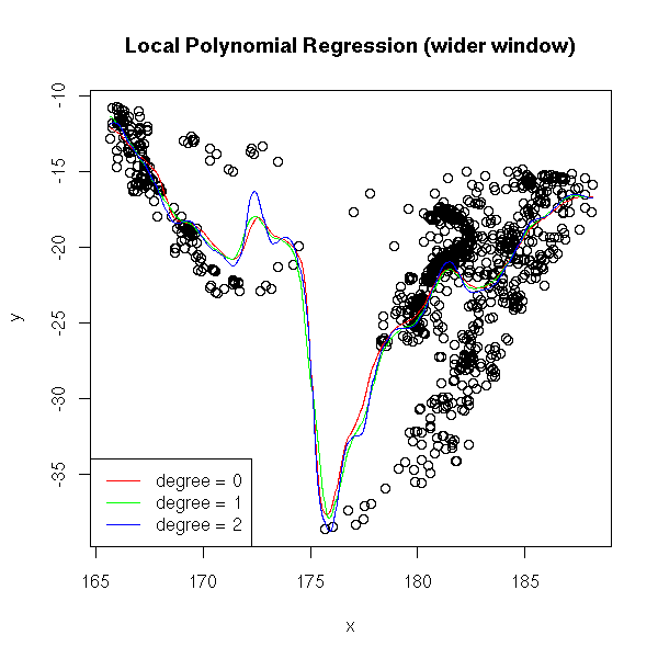
The Moving Average (aka Nadaraya-Watson regression) is biased at the ends of the domain; local linear regression (aka kernel regression) is biased when the curvature is high.
You can check this on simulated data: in the following example, the degree-0 local polynomial regression is far from the sample values.
n <- 50
x <- runif(n)
f <- function (x) { cos(3*x) + cos(5*x) }
y <- f(x) + .2*rnorm(n)
plot(y~x)
curve(f(x), add=T, lty=2)
bw <- dpill(x,y)
lines( locpoly(x,y,degree=0, bandwidth=bw), col='red' )
lines( locpoly(x,y,degree=1, bandwidth=bw), col='green' )
lines( locpoly(x,y,degree=2, bandwidth=bw), col='blue' )
legend( par("usr")[1], par("usr")[3], yjust=0,
        c("degree = 0", "degree = 1", "degree = 2"),
        lwd=1, lty=1,
        col=c('red', 'green', 'blue'))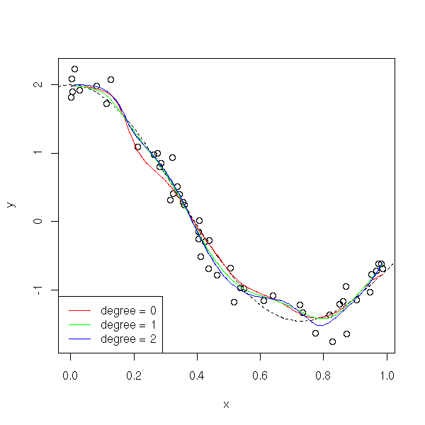
a <- locpoly(x,y,degree=0, bandwidth=bw)
b <- locpoly(x,y,degree=1, bandwidth=bw)
c <- locpoly(x,y,degree=2, bandwidth=bw)
matplot( cbind(a$x,b$x,c$x), abs(cbind(a$y-f(a$x), b$y-f(b$x), c$y-f(c$x)))^2,
         xlab='', ylab='',
         type='l', lty=1, col=c('red', 'green', 'blue') )
legend( .8*par("usr")[1]+.2*par("usr")[2], par("usr")[4], yjust=1,
        c("degree = 0", "degree = 1", "degree = 2"),
        lwd=1, lty=1,
        col=c('red', 'green', 'blue'))
title(main="MSE (Mean Square Error)")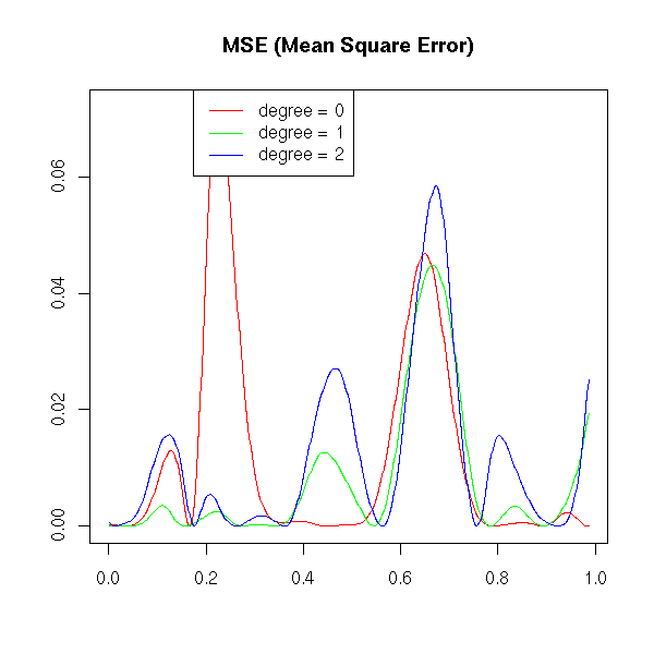
If the curve is "more curved" (if its curvature is high), higher-degree polynomial give a better approximation.
f <- function (x) { sqrt(abs(x-.5)) }
y <- f(x) + .1*rnorm(n)
plot(y~x)
curve(f(x), add=T, lty=2)
bw <- dpill(x,y)
lines( locpoly(x,y,degree=0, bandwidth=bw), col='red' )
lines( locpoly(x,y,degree=1, bandwidth=bw), col='green' )
lines( locpoly(x,y,degree=2, bandwidth=bw), col='blue' )
legend( par("usr")[1], par("usr")[3], yjust=0,
        c("degree = 0", "degree = 1", "degree = 2"),
        lwd=1, lty=1,
        col=c('red', 'green', 'blue'))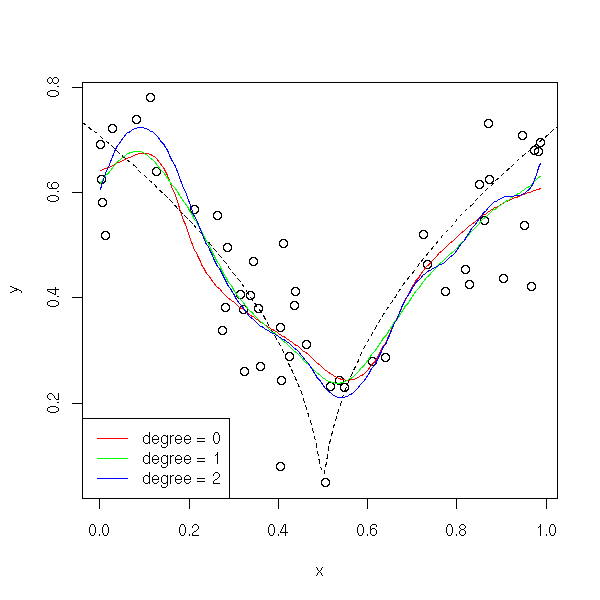
a <- locpoly(x,y,degree=0, bandwidth=bw)
b <- locpoly(x,y,degree=1, bandwidth=bw)
c <- locpoly(x,y,degree=2, bandwidth=bw)
matplot( cbind(a$x,b$x,c$x), abs(cbind(a$y-f(a$x), b$y-f(b$x), c$y-f(c$x)))^2,
         xlab='', ylab='',
         type='l', lty=1, col=c('red', 'green', 'blue') )
legend( .8*par("usr")[1]+.2*par("usr")[2], par("usr")[4], yjust=1,
        c("degree = 0", "degree = 1", "degree = 2"),
        lwd=1, lty=1,
        col=c('red', 'green', 'blue'))
title(main="MSE (Mean Square Error)")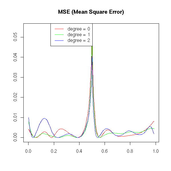
Remark: instead of using least squares for those local regressions, you could use Maximum Likelihood methods.
TODO: what is the difference? the benefit?
There are many other similar functions:
loess (modreg)         local polynomial regression, with a ticubic kernel
                       (if you do not know what to choose, choose this one)
lowess (base)
locpoly (KernSmooth)   local polynomial regression, with a gaussian
                       kernel, whise degree you can choose.
smooth (eda)           With medians
supsmu (modreg)
density (base)
On particular, one uses thes regressions to see if a linear model is a good idea or not.
# It is linear
library(modreg)
n <- 10
op <- par(mfrow=c(2,2))
for (i in 1:4) {
  x <- rnorm(n)
  y <- 1-2*x+.3*rnorm(n)
  plot(y~x)
  lo <- loess(y~x)
  xx <- seq(min(x),max(x),length=100)
  yy <- predict(lo, data.frame(x=xx))
  lines(xx,yy, col='red')
  lo <- loess(y~x, family='sym')
  xx <- seq(min(x),max(x),length=100)
  yy <- predict(lo, data.frame(x=xx))
  lines(xx,yy, col='red', lty=2)
  lines(lowess(x,y),col='blue',lty=2)
#  abline(lm(y~x), col='green')
#  abline(1,-2, col='green', lty=2)
}
par(op)
# It is not linear
n <- 10
op <- par(mfrow=c(2,2))
for (i in 1:4) {
  x <- rnorm(n)
  y <- x*(1-x)+.3*rnorm(n)
  plot(y~x)
  lo <- loess(y~x)
  xx <- seq(min(x),max(x),length=100)
  yy <- predict(lo, data.frame(x=xx))
  lines(xx,yy, col='red')
  lo <- loess(y~x, family='sym')
  xx <- seq(min(x),max(x),length=100)
  yy <- predict(lo, data.frame(x=xx))
  lines(xx,yy, col='red', lty=2)
  lines(lowess(x,y),col='blue',lty=2)
#  curve(x*(1-x), add = TRUE, col = "green", lty=2)
}
par(op)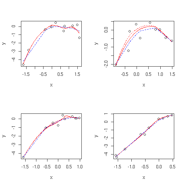
Least Squares are not the only method of approximating a function Y=f(X): here are a few others.
Instead of miniming
Sum ( y_i - a - b x_i ) ^ 2
 i
we replace the squares by absolute values and minimize
Sum abs( y_i - a - b x_i )
 i

x <- cars$speed
y <- cars$dist
my.lar <- function (y,x) {
  f <- function (arg) {
    a <- arg[1]
    b <- arg[2]
    sum(abs(y-a-b*x))
  }
  r <- optim( c(0,0), f )$par
  plot( y~x )
  abline(lm(y~x), col='red', lty=2)
  abline(r[1], r[2])
  legend( par("usr")[1], par("usr")[4], yjust=1,
          c("Least Squares", "Least Absolute Values"),
          lwd=1, lty=c(2,1),
          col=c(par('fg'),'red'))
}
my.lar(y,x)
TODO:
library(quantreg)
?rq
In least squares, we try to minimize
Sum( rho( (yi - \hat yi) / sigma ) )
 i
where \hat yi = a + b xi and rho(x) = x^2. M-estimators are estimators obtained with a different choice of the "rho" function. For instance, in L1 regression, we just set rho(x)=abs(x). Huber regression is between Least Squares and L1-regression: we still try to minimize this sum, but now with
rho(x) = x^2/2                if abs(x) <= c
         c * abs(x) - c^2/2   otherwise
(where c is chosen arbitrarily, proportionnal to a robust estimator of the noise median).
On can also interpret Huber regression as a weighted regression, in which the weights are
w(u) = 1          if abs(u) < c
       c/abs(u)   else
This regression is useful if the error term distribution is very dispersed.
In R, Huber regression is achieved by the "rlm" function, in the "MASS" package.
In the following example, we remark that Huber regression is not very resistant: with outliers, it gives the same result as classical regression.
library(MASS)
n <- 20
x <- rnorm(n)
y <- 1 - 2*x + rnorm(n)
y[ sample(1:n, floor(n/4)) ] <- 10
plot(y~x)
abline(1,-2,lty=3)
abline(lm(rlm(y~x)), col='red')
abline(lm(y~x), lty=3, lwd=3)

On the contrary, it is supposed to be robustL
TODO (recall that in the following situation, one would first try to
transform the data to make them more "gaussian")

n <- 100
x <- rnorm(n)
y <- 1 - 2*x + rcauchy(n,1)
plot(y~x)
abline(1,-2,lty=3)
abline(lm(rlm(y~x)), col='red')
abline(lm(y~x), lty=3, lwd=3)

TODO: understand. Compare with the following plot

#library(lqs)   # now merged into MASS
x <- rnorm(20)
y <- 1 - x + rnorm(20)
x <- c(x,10)
y <- c(y,1)
plot(y~x)
abline(1,-1, lty=3)
abline(lm(y~x))
abline(rlm(y~x, psi = psi.bisquare, init = "lts"), col='orange',lwd=3)
abline(rlm(y~x), col='red')
abline(rlm(y~x, psi = psi.hampel, init = "lts"), col='green')
abline(rlm(y~x, psi = psi.bisquare), col='blue')
title(main='Huber regression (rlm)')

We no longer try to minimize the sum of all the squared error, but just the sum of the smallest squared errors. If you want exact computations, it will be time-consuming (if there are n observations and if you want to remoce k of them, you have to consider all the sets of n-k observations and retain the one with the smallest sum of squares) -- we shall therefore use an empirical, approximate method.
?ltsreg

n <- 100
x <- rnorm(n)
y <- 1 - 2*x + rnorm(n)
y[ sample(1:n, floor(n/4)) ] <- 7
plot(y~x)
r1 <- lm(y~x)
r2 <- lqs(y~x, method='lts')
abline(r1, col='red')
abline(r2, col='green')
abline(1,-2,lty=3)
legend( par("usr")[1], par("usr")[3], yjust=0,
        c("Linear regression", "Trimmed regression"),
        lty=1, lwd=1,
        col=c("red", "green") )
title("Least Trimmed Squares (LTS)")
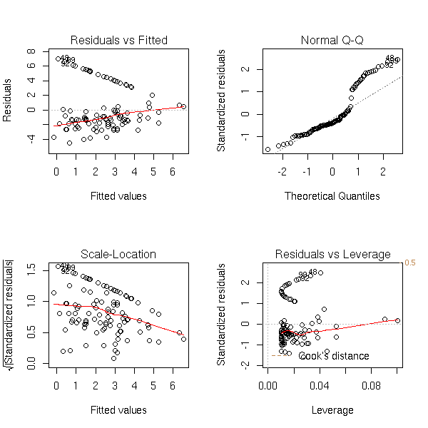
If you just look at the classical regression diagnosis plots, you do not see anything...
TODO...

op <- par(mfrow=c(2,2))
plot(r1)
par(op)
TODO: estimate the error with bootstrap
This is a resistant regression.
Trimmed regression has several variants:
lqs: it is almost a normal regression, but instead of minimizing the
sum of all the squared residuals, we sort them and minimize the
middle one.

lqs(..., method='lms'): idem, but with the residual number
"floor(n/2) + floor((p+1)/2)" where n is the number of observations
and p the number of predictive variables.

lqs(..., method='S'): dunno.
TODO
This generalization of the Least Squares method tackles the problem of correlated and/or heteroskedastic (it means "different variances") errors. More about this later.
The least squares method assumes that the error term (the noise) is made of idenpendant gaussian variables, of the same variance. Generalized Least Squares tackle the case of different variances (but you have to know the variances), non-gaussian noises (e.g., asymetric), non-independant noises (e.g., with time series: but you have to choose a model to describe this dependancy).
We shall detail those situations later in this document
TODO: where???
library(MASS)
?lm.gls
library(nlme)
?gls
TODO: read...
The weighted least squares method consists to compute the regression, the residuals, to assign a weight to the observations (low weight for high residuals) and to perform a new regression.
# Evil data...
n <- 10
x <- rnorm(n)
y <- 1 - 2*x + rnorm(n)
x[1] <- 5
y[1] <- 0
my.wls <- function (y,x) {
  # A first regression
  r <- lm(y~x)$residuals
  # The weights
  w <- compute.weights(r)
  # A new regression
  lm(y~x, weights=w)
}
compute.weights <- function (r) {
  # Compute the weights as you want, as long as they are positive,
  # sum up to 1 and the high-residuals have low weights.
  # My choice might be neither standard nor relevant.
  w <- r*r
  w <- w/mean(w)
  w <- 1/(1+w)
  w <- w/mean(w)
}
plot(y~x)
abline(1,-2, lty=3)
abline(lm(y~x))
abline(my.wls(y,x), col='red')
title(main="Weighted Regression")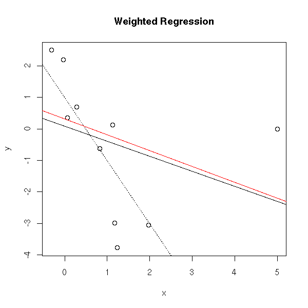
Weighted least squares can be seen as a standard regression after data transformation: it has a purely geometric interpretation.
# Situation in which you would like to use weighted least squares
N <- 500
x <- runif(N)
y <- 1 - 2 * x + (2 - 1.5 * x) * rnorm(N)
op <- par(mar = c(1,1,3,1))
plot(y ~ x, axes = FALSE,
     main = "Weighted least squares")
box()
for (u in seq(-3,3,by=.5)) {
  segments(0, 1 + 2 * u, 1, -1 + .5 * u,
           col = "blue")
}
abline(1, -2, col = "blue", lwd = 3)
par(op)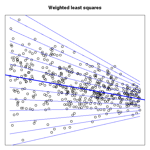
We do the same as Weighted Least Squares (WLS), but we iterate until the results stabilize.
my.irls.plot <- function (y,x, n=10) {
  plot(y~x)
  abline(lm(y~x))
  r <- lm(y~x)$residuals
  for (i in 1:n) {
    w <- compute.weights(r)
    print(w)
    r <- lm(y~x, weights=w)
    abline(r, col=topo.colors(n)[i], lwd=ifelse(i==n,3,1))
    r <- r$residuals
  }
  lm(y~x, weights=w)
}
my.irls.plot(y,x)
abline(1,-2, lty=3)
abline(my.wls(y,x), col='blue', lty=3, lwd=3)
title(main="Iteratively Reweighted Least Squares")
TODO: IRLS
plot( weights ~ residuals )
It is a bell-shaped on which we see the "influent" points (their
weight is low). We can try to compute a new regression without those
points. If the results are different, it is a bad sign...
The idea behind regression of a variable Y against a variable X is simply to find the function
f(x) = E[ Y | X=x ].
If we knew the joint distribution of (X,Y), we could exactly compute this regression function -- but we only have a sample, so we try to estimate it by assuming that it has a simple form.
Similarly, median regression (aka L^1 regression or LAD regression) focuses on the conditionnal median,
f(x) = Median[ Y | X=x ].
Instead of the median, we can consider any quantile (typically, we shall consider several quantiles, say all the quartiles, or all the deciles) and focus on
f(x) = tau-th quantile of ( Y | X=x ).
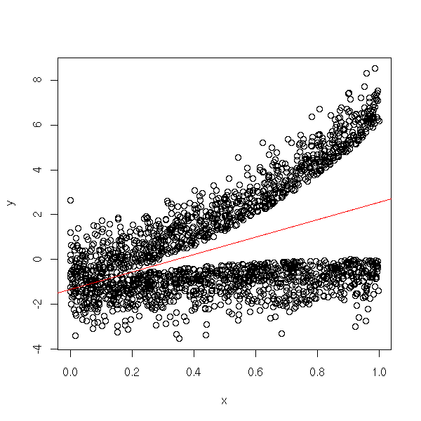
Instead of having a single line or a single curve, we get several -- this allows us to spot (and measure) phenomena such as heteroskedasticity or even the bimodality of Y|X=x for some values of x.
But how do we compute it? The mean of y1,...,yn can be defined as the real mu that minumizes
Sum( (y_i - mu)^2 ).
 i
Similarly, the median is a real that minimizes
Sum( abs(y_i - m) ).
 i
For the tau-th quantile (where tau is in the interval (0,1): the 0th quantile is the minimum, the .25-th quantile is the first quartile, the .5-th quantile is the median, etc.), we can minimize
Sum( r_tau( y_i - q ) )
 i
where r_tau is the function
r_tau(x) = tau * x         if x >= 0
           (tau - 1) * x   if x < 0
You can check that r_.5 is the absolute value (well, half the absolute value).
op <- par(mfrow=c(2,2), mar=c(2,4,4,2))
r <- function (tau, x) { ifelse(x<0, (tau-1)*x, tau*x) }
curve(r(0,x), xlim=c(-1,1), ylim=c(0,1), lwd=3, main="Minimum", xlab="")
abline(0,1,lty=2)
abline(0,-1,lty=2)
abline(h=c(0,.25,.5,.75), lty=3)
curve(r(.25,x), xlim=c(-1,1), ylim=c(0,1), lwd=3, main="First quartile")
abline(0,1,lty=2)
abline(0,-1,lty=2)
abline(h=c(0,.25,.5,.75), lty=3)
curve(r(.5,x), xlim=c(-1,1), ylim=c(0,1), lwd=3, main="Median")
abline(0,1,lty=2)
abline(0,-1,lty=2)
abline(h=c(0,.25,.5,.75), lty=3)
curve(r(.75,x), xlim=c(-1,1), ylim=c(0,1), lwd=3, main="Third quartile")
abline(0,1,lty=2)
abline(0,-1,lty=2)
abline(h=c(0,.25,.5,.75), lty=3)
par(op)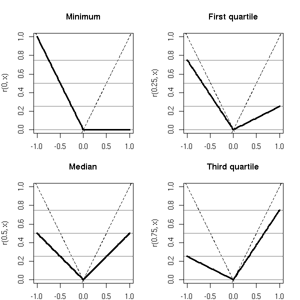
Let us now switch from the mean, median or quantile computation to the mean, median or quantile regression. OLS (mean) regression find a and b that minimize
Sum( (y_i - (a + b * x))^2 ).
 i
Median regression finds a and b that minimize
Sum( abs(y_i - (a + b * x)) ).
 i
Similarly, quantile regression (for a given tau -- and you will want to consider several) finds a and b that minimizes
Sum( r_tau(y_i - (a + b * x)) ).
 i
From a computationnal point of view, this can be expressed as a Linear Program -- one can solve it with algorithms such as the simplex.
TODO: understand how it becomes a linear program.
It is high time for a few examples.
TODO: find some data...

N <- 2000
x <- runif(N)
y <- rnorm(N)
y <- -1 + 2 * x + ifelse(y>0, y+5*x^2, y-x^2)
plot(x,y)
abline(lm(y~x), col="red")
library(quantreg)
plot(y~x)
for (a in seq(.1,.9,by=.1)) {
  abline(rq(y~x, tau=a), col="blue", lwd=3)
}
plot(y~x)
for (a in seq(.1,.9,by=.1)) {
  r <- lprq(x,y,
            h=bw.nrd0(x),  # See ?density
            tau=a)
  lines(r$xx, r$fv, col="blue", lwd=3)
}
op <- par(mar=c(3,2,4,1))
r <- rq(y~x, tau=1:49/50)
plot(summary(r), nrow=1)
par(op)
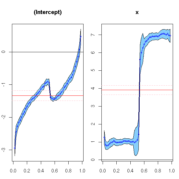
How do we interpret those plots? Let us look at more "normal" data: the intercept of the quantile regression correspond to the noise quantiles; the slope should be constant.
y <- -1 + 2 * x + rnorm(N)
op <- par(mar=c(3,2,4,1))
r <- rq(y~x, tau=1:49/50)
plot(summary(r), nrow=1)
par(op)

TODO:
plot(rq(..., tau=1:99/100)
TODO
?anova.rq   # To compare models?
?nlrq       # For non-linear models

# 2-dimensionnal kernel estimation?
# (this uses the akima and tripack packages, that are not free)
plot( rqss( z ~ qss(cbind(x,y), lambda=0.8) ) )

TODO
library(quantreg)
?rq
rq(y~x, tau=.5) # Median regression
?table.rq
http://www.econ.uiuc.edu/~econ472/tutorial15.html
# library(lqs)   # now part of MASS
n <- 100
x <- rnorm(n)
y <- 1 - 2*x + rnorm(n)
y[ sample(1:n, floor(n/4)) ] <- 7
plot(y~x)
abline(1,-2,lty=3)
r1 <- lm(y~x)
r2 <- lqs(y~x, method='lts')
r3 <- lqs(y~x, method='lqs')
r4 <- lqs(y~x, method='lms')
r5 <- lqs(y~x, method='S')
abline(r1, col='red')
abline(r2, col='green')
abline(r3, col='blue')
abline(r4, col='orange')
abline(r5, col='purple')
legend( par("usr")[1], par("usr")[3], yjust=0,
        c("Linear Regression", "LTS",
        "lqs", "lms", "S"),
        lty=1, lwd=1,
        col=c("red", "green", "blue", "orange", "purple") )
title("LTS and variants")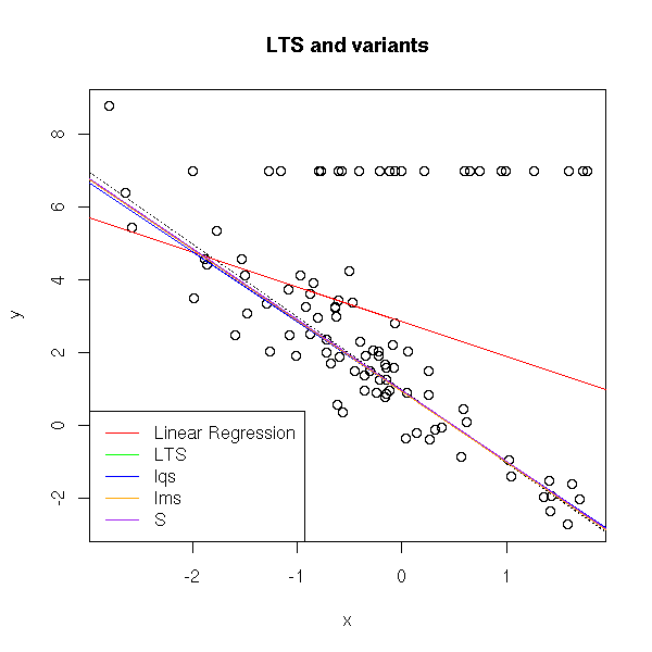
A regression is said to be resistant if it is not very sensitive to outliers. It is robust if it remains valid when its asumptions (often, gaussian data, homoscedasticity, independance) are no longer satisfied.
We have already seen some examples, such as trimmed regression (lqs) or Huber regression (rlm). Here are a few others -- I shall not dive into the details.
TODO: modify those examples to get a comparison of those different
regressions, in various situations (one outliers, several outliers,
non-gaussian predictive variable, non-normal errors).
TODO: idem with non-linear regressions.

# Example
x <- rnorm(20)
y <- 1 - x + rnorm(20)
x <- c(x,10)
y <- c(y,1)
plot(y~x)
abline(lm(y~x), col='blue')
title(main="Classical regression")
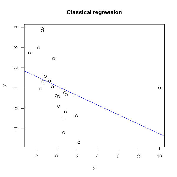
# How bad usual regression is
plot(lm(y~x), which=4,
     main="Cook's distance")
plot(y~x)
for (i in 1:length(x))
  abline(lm(y~x, subset= (1:length(x))!=i ), col='red')
title(main="Classical regression minus one point")
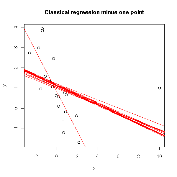
# line (in the eda package)
library(eda)
plot(y~x)
abline(1,-1, lty=3)
abline(lm(y~x))
abline(coef(line(x,y)), col='red')
title(main='"line", in the "eda" package')

# Trimmed regression
#library(lqs)
plot(y~x)
abline(1,-1, lty=3)
abline(lm(y~x))
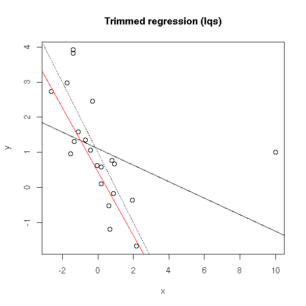
abline(lqs(y~x), col='red')
title(main='Trimmed regression (lqs)')
# glm (from the manual, it should be IWLS, but we get the same
# result...)
plot(y~x)
abline(1,-1, lty=3)
abline(lm(y~x))
abline(glm(y~x), col='red')
title(main='"glm" regression')

plot(y~x)
abline(1,-1, lty=3)
abline(lm(y~x))
abline(rlm(y~x, psi = psi.bisquare, init = "lts"), col='orange',lwd=3)
abline(rlm(y~x), col='red')
abline(rlm(y~x, psi = psi.hampel, init = "lts"), col='green')
abline(rlm(y~x, psi = psi.bisquare), col='blue')
title(main='Huber regression (rlm)')

You will usually use those robust regressions as follows: perform a linear regression and a robust one; if the coincide, use the linear regression; if they do not, try to find why (it is a bad omen).
TODO: Introduction. In particular, explain what PCR and PLS are here: compare them with ridge regression.
This is a regression on the first principal components (see "Principal Component Analysis (PCA)", somewhere in this document) of the predictive variables.
You can compute it by hand.
# The change-of-base matrix
e <- eigen(cor(x)))
# Normalize x and perform the change of base
enx <- scale(x) %*% e$vec
# Regression on those new vectors
lm(y ~ enx)
More directly:
lm(y ~ princomp(x)$scores)
If you just want the first three variables:
lm(y ~ princomp(x)$scores[,1:3])
Interpreting the new coordinates requires some work/thinking -- but the "biplot(princomp(x))" command will help you.
You can replace the Principal Component Analysis (PCA) by an Independant Component Analysis, thereby obtaining an "Independant Component Regression" -- if your data are not gaussian, this may work.
TODO: URL
Independant variable selection: application of independant
component analysis to forecasting a stock index
There is, however, a slight problem: when we chose the new basis, we only looked at the predictive variables x, not the variable to predict y: but some of the predictive variables might appear irrelevant in the PCA and nonetheless be tightly linked to y -- or, conversely, some predictive variables might seem pivotal from the PCA while being irrelevant (orthogonal) to the variable to predict.
Partial Least Squares (PLS) tackle this problem: it is a regression on a new basis, that looks like a principal component analysis computed "with respect to" the variable to predict y.
library(help=pls)
library(pls)
?simpls.fit
TODO: understand...
On Internet, you can find the following algorithm to compute the PCA
from NIPALS (Non-Llinearly Iterated PArtial Least Squares).
(t=scores, p=loadings)

begin loop
  select a proxy t-vector (any large column of X)
  small = 10^(-6) (e.g.)
  begin loop
    p = X'*t
    p is normalised to length one: abs(p)=1
    t = X*p
  end loop if convergence: (t_new - t_old) << small
  remove the modelled information from X: X_new = X_old - t*p'
end loop (if all PCs are calculated)
http://www.bitjungle.com/~mvartools/muvanl/

PLS = somewhere between classical ("multiple") regression and
principal component regression. You can also imagine other methods
inbetween (by changing the value of a parameter: 0 for linear
regression, 1 for principal component regression, 0.5 for PLS).

PCR: Factors from X'X
PLS: Factors from Y'XX'Y
The difference between PCR and PLS is the way factor scores are extracted.

Remark: multi-way data analysis
This is stil "linear algebra", but with 3-dimensional arrays (or
more) instead of 2-dimensional matrices.
There is a "pls" library:
http://cran.r-project.org/src/contrib/Devel/
http://www.gsm.uci.edu/~joelwest/SEM/PLS.html

library(help="pls.pcr")
Least Squares Regression looks for a function f that minimizes
RSS(f) = Sum (y_i - f(x_i))^2
          i
But this can yield "naughty", pathological functions. To stay in the realm of "nice" functions, we can add a term
PRSS(f) = Sum (y_i - f(x_i))^2  + lambda J(f)
           i
where J increases with the "naughtiness" of the function and lambda is a user-chosen positive real. For instamce, if you want functions whose curvature (i.e., second derivative) is not too high, you can choose
J(f) = \int f''^2
(actually, one can define splines like that).
Classical regression computes
b = (X'X)^-1 X' y.
The problem is that sometimes, when the data are multicolinear (i.e., if some of the predictive variables are (almost) linearly dependant, for instance if X1 = X2 + X3 (if X2 is almost equal to X2 + X3)), then the X'X matrix is (almost) singular: the resulting estimator has a very high variance. You can circumvent the problem by shifting all the eigen values of the matrix and by computing
b = (X'X + kI)^-1 X' y.
This reduces the variance -- but, of course, the resulting estimator is biased. If the reduction invariance is higher than the increase in bias, the Mean Square Error (MSE) decreases and this new estimator is worthy of our interest.
You can also see ridge regression as a penalized regression: instead of looking for a b that minimizes
Sum( y_i - b0 - Sum( xij bj ) )^2
 i               j
you look for a b that minimizes
Sum( y_i - b0 - Sum( xij bj ) )^2 + k Sum bj^2
 i               j                     j>0
This avoids overly large coefficients (this is waht happens with multicolinearity: you can have one large positive coefficient compensated by a large negative one).
It is equivalent to look for a b that minimizes
Sum( y_i - b0 - Sum( xij bj ) )^2
 i               j
under the condition
Sum bj^2 <= s
j>0
The problem is then to choose the value of k (or s) so that the variance be low and the bias not too high: you can use heuristics, graphics or crossed validation -- none of those methods are satisfactory.
Practically, we first center and normalize the columns of X -- there will be no constant term. You could program ot yourself:
my.lm.ridge <- function (y, x, k=.1) {
  my <- mean(y)
  y <- y - my
  mx <- apply(x,2,mean)
  x <- x - matrix(mx, nr=dim(x)[1], nc=dim(x)[2], byrow=T)
  sx <- apply(x,2,sd)
  x <- x/matrix(sx, nr=dim(x)[1], nc=dim(x)[2], byrow=T)
  b <- solve( t(x) %*% x + diag(k, dim(x)[2]), t(x) %*% y)
  c(my - sum(b*mx/sx) , b/sx)
}
or using the definition in terms of penalized least squares:
my.ridge <- function (y,x,k=0) {
  xm <- apply(x,2,mean)
  ym <- mean(y)
  y <- y - ym
  x <- t( t(x) - xm )
  ss <- function (b) {
    t( y - x %*% b ) %*% ( y - x %*% b ) + k * t(b) %*% b
  }
  b <- nlm(ss, rep(0,dim(x)[2]))$estimate
  c(ym-t(b)%*%xm, b)
}
my.ridge.test <- function (n=20, s=.1) {
  x <- rnorm(n)
  x1 <- x + s*rnorm(n)
  x2 <- x + s*rnorm(n)
  x <- cbind(x1,x2)
  y <- x1 + x2 + 1 + rnorm(n)
  lambda <- c(0, .001, .01, .1, .2, .5, 1, 2, 5, 10)
  b <- matrix(nr=length(lambda), nc=1+dim(x)[2])
  for (i in 1:length(lambda)) {
    b[i,] <- my.ridge(y,x,lambda[i])
  }
  plot(b[,2], b[,3],
       type="b",
       xlim=range(c(b[,2],1)), ylim=range(c(b[,3],1)))
  text(b[,2], b[,3], lambda, adj=c(-.2,-.2), col="blue")
  points(1,1,pch="+", cex=3, lwd=3)
  points(b[8,2],b[8,3],pch=15)
}
my.ridge.test()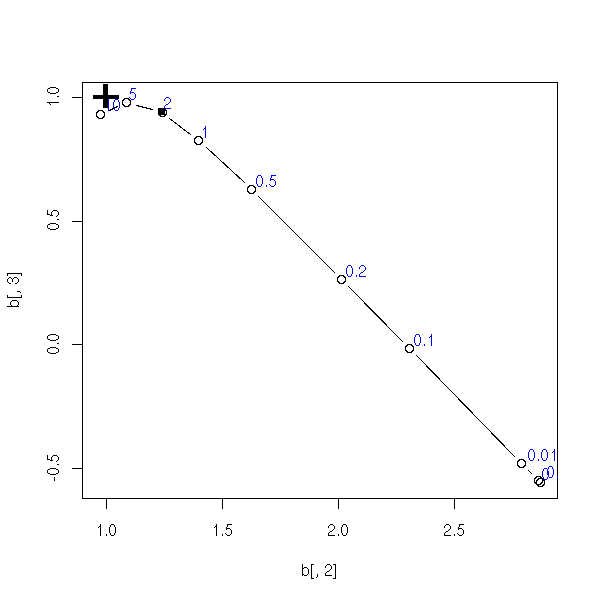
TODO: Add a title to this plot
(ridge regression and multicolinearity)
op <- par(mfrow=c(3,3))
for (i in 1:9) {
  my.ridge.test()
}
par(op)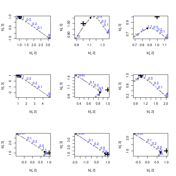
TODO: Add a title to this plot
(ridge regression and milder multicolinearity)
op <- par(mfrow=c(3,3))
for (i in 1:9) {
  my.ridge.test(20,10)
}
par(op)
But there is already a "lm.ridge" function in the "MASS" package: we shall use it.
Let us first remark (as we stated above) that in some cases (here, multicolinearity), the variance of the regression coefficients is very high. On the contrary, that of the ridge regression coefficients is lower -- but they are biased.
my.sample <- function (n=20) {
  x <- rnorm(n)
  x1 <- x + .1*rnorm(n)
  x2 <- x + .1*rnorm(n)
  y <- 0 + x1 - x2 + rnorm(n)
  cbind(y, x1, x2)
}

n <- 500
r <- matrix(NA, nr=n, nc=3)
s <- matrix(NA, nr=n, nc=3)
for (i in 1:n) {
  m <- my.sample()
  r[i,] <- lm(m[,1]~m[,-1])$coef
  s[i,2:3] <- lm.ridge(m[,1]~m[,-1], lambda=.1)$coef
  s[i,1] <- mean(m[,1])
}
plot( density(r[,1]), xlim=c(-3,3),
      main="Multicolinearity: high variance")
abline(v=0, lty=3)
lines( density(r[,2]), col='red' )
lines( density(s[,2]), col='red', lty=2 )
abline(v=1, col='red', lty=3)
lines( density(r[,3]), col='blue' )
lines( density(s[,3]), col='blue', lty=2 )
abline(v=-1, col='blue', lty=3)
# We give the mean, to show that it is biased
evaluate.density <- function (d,x, eps=1e-6) {
  density(d, from=x-eps, to=x+2*eps, n=4)$y[2]
}
x<-mean(r[,2]); points( x, evaluate.density(r[,2],x) )
x<-mean(s[,2]); points( x, evaluate.density(s[,2],x) )
x<-mean(r[,3]); points( x, evaluate.density(r[,3],x) )
x<-mean(s[,3]); points( x, evaluate.density(s[,3],x) )
legend( par("usr")[1], par("usr")[4], yjust=1,
        c("intercept", "x1", "x2"),
        lwd=1, lty=1,
        col=c(par('fg'), 'red', 'blue') )
legend( par("usr")[2], par("usr")[4], yjust=1, xjust=1,
        c("classical regression", "ridge regression"),
        lwd=1, lty=c(1,2),
        col=par('fg') )
We can compute the mean and variance of our estimators:
# LS regression
> apply(r,2,mean)
[1] -0.02883416  1.04348779 -1.05150408
> apply(r,2,var)
[1] 0.0597358 2.9969272 2.9746692

# Ridge regression
> apply(s,2,mean)
[1] -0.02836816  0.62807824 -0.63910220
> apply(s,2,var)
[1] 0.05269393 0.99976908 0.99629095
But we cannot compare them that way; to do so, we prefer using the Mean Square Error (MSE): it is the mean of the squares of the differences of the real value of the looked-for parameter (while the variance is defined in a similar way, with the mean instead of the real value).
TODO: give a formula, it might be clearer.

> v <- matrix(c(0,1,-1), nr=n, nc=3, byrow=T)
> apply( (r-v)^2, 2, mean )
[1] 0.06044774 2.99282451 2.97137250
> apply( (s-v)^2, 2, mean )
[1] 0.05339329 1.13609534 1.12454560
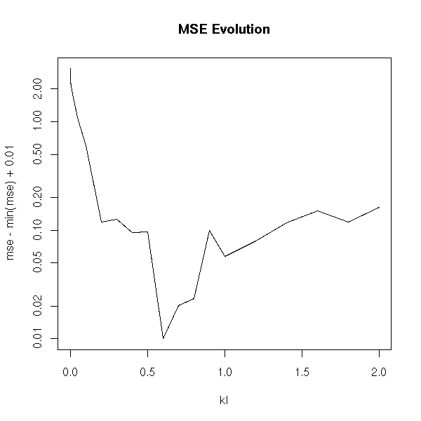
We can plot the evolution of this MSE with k:
n <- 500
v <- matrix(c(0,1,-1), nr=n, nc=3, byrow=T)
mse <- NULL
kl <- c(1e-4, 2e-4, 5e-4,
        1e-3, 2e-3, 5e-3,
        1e-2, 2e-2, 5e-2,
        .1,  .2,  .3,  .4,  .5,  .6,  .7,  .8,  .9,
        1,  1.2, 1.4, 1.6, 1.8,   2)
for (k in kl) {
  r <- matrix(NA, nr=n, nc=3)
  for (i in 1:n) {
    m <- my.sample()
    r[i,2:3] <- lm.ridge(m[,1]~m[,-1], lambda=k)$coef
    r[i,1] <- mean(m[,1])
  }
  mse <- append(mse, apply( (r-v)^2, 2, mean )[2])
}
plot( mse ~ kl, type='l' )
title(main="MSE evolution")
With a logarithmic scale:
plot( mse-min(mse)+.01 ~ kl, type='l', log='y' )
title(main="MSE Evolution")
With ranks:
plot( rank(mse) ~ kl, type='l' )
title(main="MSE Evolution")
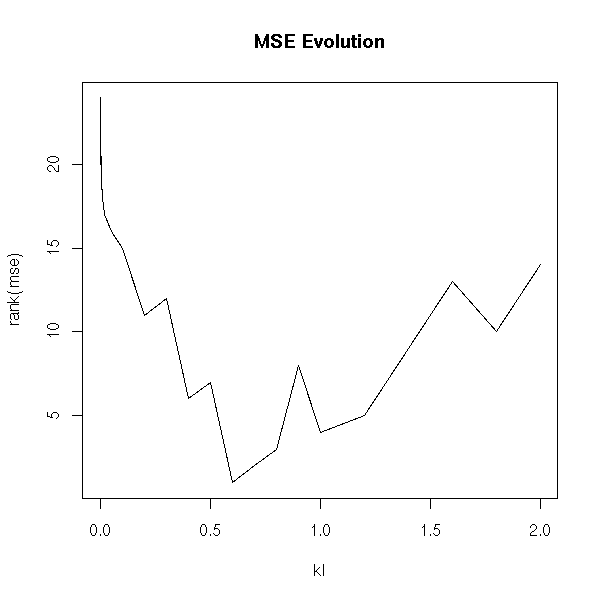
On this example, we see that k=0.5 is a good value (but according to the literature, it is VERY high: they say you should not go beyond 0.1...)
The problem is that usually you cannot compute the MSE: you would have to know the exact values of the parameters -- the very quantities we strive to estimate.
You can also choose k from a plot: say, the parameters (or something that depends on the parameters, such as R^2) with respect to k.
m <- my.sample()
b <- matrix(NA, nr=length(kl), nc=2)
for (i in 1:length(kl)) {
  b[i,] <- lm.ridge(m[,1]~m[,-1], lambda=kl[i])$coef
}
matplot(kl, b, type="l")
abline(h=c(0,-1,1), lty=3)
# Heuristic estimation for k...
k <- min( lm.ridge(m[,1]~m[,-1], lambda=kl)$GCV )
abline(v=k, lty=3)
title(main="Bias towards 0 in ridge regression")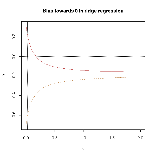
It might be clearer with a logarithmic scale:
m <- my.sample()
b <- matrix(NA, nr=length(kl), nc=2)
for (i in 1:length(kl)) {
  b[i,] <- lm.ridge(m[,1]~m[,-1], lambda=kl[i])$coef
}
matplot(kl, b, type="l", log='x')
abline(h=c(0,-1,1), lty=3)
k <- min( lm.ridge(m[,1]~m[,-1], lambda=kl)$GCV )
abline(v=k, lty=3)
title(main="Bias towards 0 in ridge regression")
The estimators are more and more biased (towards 0) when k becomes large: in this example, a value between 0.01 and 0.1 would be fine -- perhaps.
my.lm.ridge.diag <- function (y, x, k=.1) {
  my <- mean(y)
  y <- y - my
  mx <- apply(x,2,mean)
  x <- x - matrix(mx, nr=dim(x)[1], nc=dim(x)[2], byrow=T)
  sx <- apply(x,2,sd)
  x <- x/matrix(sx, nr=dim(x)[1], nc=dim(x)[2], byrow=T)
  b <- solve( t(x) %*% x + diag(k, dim(x)[2]), t(x) %*% y)
  v <- solve( t(x) %*% x + diag(k, dim(x)[2]),
       t(x) %*% x %*% solve( t(x) %*% x + diag(k, dim(x)[2]),
       diag( var(y), dim(x)[2] ) ))
  ss <- t(b) %*% t(x) %*% y
  list( b = b, varb = v, ss = ss )
}

m <- my.sample()
b <- matrix(NA, nr=length(kl), nc=2)
v <- matrix(NA, nr=length(kl), nc=1)
ss <- matrix(NA, nr=length(kl), nc=1)
for (i in 1:length(kl)) {
  r <- my.lm.ridge.diag(m[,1], m[,-1], k=kl[i])
  b[i,] <- r$b
  v[i,] <- sum(diag(r$v))
  ss[i,] <- r$ss
}
matplot(kl, b,
        type="l", lty=1, col=par('fg'), axes=F, ylab='')
axis(1)
abline(h=c(0,-1,1), lty=3)
par(new=T)
matplot(kl, v, type="l", col='red', axes=F, ylab='')
par(new=T)
matplot(kl, ss, type="l", col='blue', axes=F, ylab='')
legend( par("usr")[2], par("usr")[4], yjust=1, xjust=1,
        c("parameters", "variance", "sum of squares"),
        lwd=1, lty=1, col=c(par('fg'), "red", "blue") )
matplot(log(kl), b,
        type="l", lty=1, col=par('fg'), axes=F, ylab='')
axis(1)
abline(h=c(0,-1,1), lty=3)
par(new=T)
matplot(log(kl), v, type="l", col='red', axes=F, ylab='')
par(new=T)
matplot(log(kl), ss, type="l", col='blue', axes=F, ylab='')
# I cannot put the legend if the scale is logarithmic...
legend( par("usr")[1],
        .9*par("usr")[3] + .1*par("usr")[4],
        yjust=0, xjust=0,
        c("parameters", "variance", "sum of squares"),
        lwd=1, lty=1, col=c(par('fg'), "red", "blue") )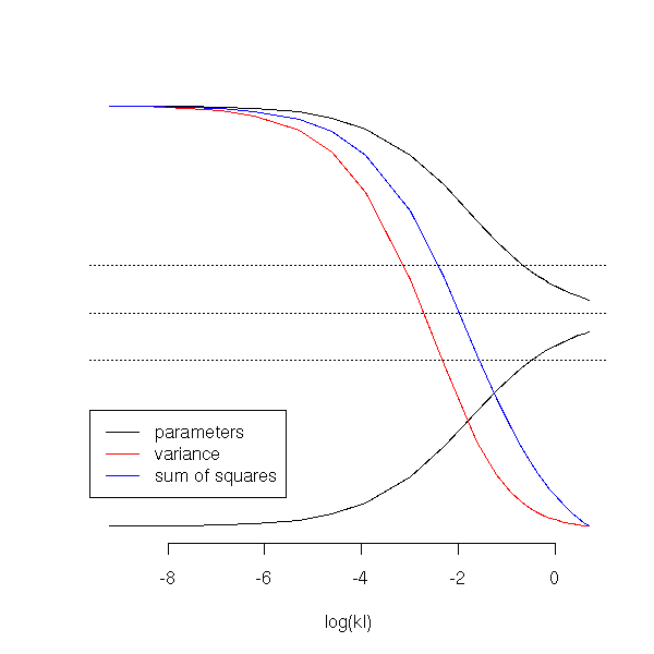
TODO: add R^2 to the preceding plot
Actually, if you look at several such simulations, you will see that those plots are not helpful at all: the curves all have the same shape, but the exact values of the parameters can be anywhere...
op <- par(mfrow=c(3,3))
for (j in 1:9) {
  m <- my.sample()
  b <- matrix(NA, nr=length(kl), nc=2)
  for (i in 1:length(kl)) {
    b[i,] <- lm.ridge(m[,1]~m[,-1], lambda=kl[i])$coef
  }
  matplot(kl, b, type="l", log='x')
  abline(h=c(0,-1,1), lty=3)
  k <- min( lm.ridge(m[,1]~m[,-1], lambda=kl)$GCV )
  abline(v=k, lty=3)
}
par(op)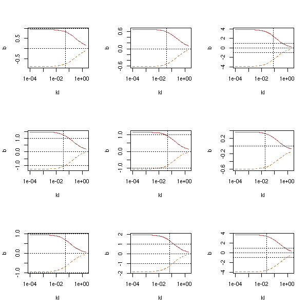
To choose the value of k, you can also use cross-valudation.
m <- my.sample()
N <- 20
err <- matrix(nr=length(kl), nc=N)
for (j in 1:N) {
  s <- sample(dim(m)[1], floor(3*dim(m)[1]/4))
  mm <- m[s,]
  mv <- m[-s,]
  for (i in 1:length(kl)) {
    r <- lm.ridge(mm[,1]~mm[,-1], lambda=kl[i])
    # BUG...
    b <- r$coef / r$scales
    a <- r$ym - t(b) %*% r$xm
    p <- rep(a, dim(mv)[1]) + mv[,-1] %*% b
    e <- p-mv[,1]
    err[i,j] <- sum(e*e)
  }
}
err <- apply(err, 1, mean)
plot(err ~ kl, type='l', log='x')
TODO: there is a problem with this code.
(we try to minimize the error, that should grow with k...)
Finally, you can use the various heuristics provided by the "lm.ridge" command.
m <- my.sample()
x <- m[,1]
y <- m[,-1]

r <- lm.ridge(y~x, lambda=kl);
r$kHKB; r$kLW; min(r$GCV)
Fir this example:
[1] 0
[1] 0
[1] 0.04624034
The computer advises us to use classical regression -- but we have seen above that, on this example, k=0.5 was a good value...
Other example:
data(longley)
y <- longley[,1]
x <- as.matrix(longley[,-1])
r <- lm.ridge(y~x, lambda=kl);
r$kHKB; r$kLW; min(r$GCV)
This yields:
[1] 0.006836982
[1] 0.05267247
[1] 0.1196090
See also:
library(help=lpridge) # Local polynomial (ridge) regression.
You might want to read:
J.O. Rawlings, Applied Regression Analysis: A Research Tool (1988), chapter 12.
This is a variant of ridge regression, with an L1 constraint instead of the L2 one: we try to find b that minimizes
Sum( y_i - b0 - Sum( xij bj ) )^2 + k Sum abs(bj).
 i               j                    j>0
We could implement it by hand:
my.lasso <- function (y,x,k=0) {
  xm <- apply(x,2,mean)
  ym <- mean(y)
  y <- y - ym
  x <- t( t(x) - xm )
  ss <- function (b) {
    t( y - x %*% b ) %*% ( y - x %*% b ) + k * sum(abs(b))
  }
  b <- nlm(ss, rep(0,dim(x)[2]))$estimate
  c(ym-t(b)%*%xm, b)
}

my.lasso.test <- function (n=20) {
  s <- .1
  x <- rnorm(n)
  x1 <- x + s*rnorm(n)
  x2 <- x + s*rnorm(n)
  x <- cbind(x1,x2)
  y <- x1 + x2 + 1 + rnorm(n)
  lambda <- c(0, .001, .01, .1, .2, .5, 1, 2, 5, 10)
  b <- matrix(nr=length(lambda), nc=1+dim(x)[2])
  for (i in 1:length(lambda)) {
    b[i,] <- my.lasso(y,x,lambda[i])
  }
  plot(b[,2], b[,3],
       type = "b",
       xlim = range(c(b[,2],1)),
       ylim = range(c(b[,3],1)))
  text(b[,2], b[,3], lambda, adj=c(-.2,-.2), col="blue")
  points(1,1,pch="+", cex=3, lwd=3)
  points(b[8,2],b[8,3],pch=15)
}
my.lasso.test()
op <- par(mfrow=c(3,3))
for (i in 1:9) {
  my.lasso.test()
}
par(op)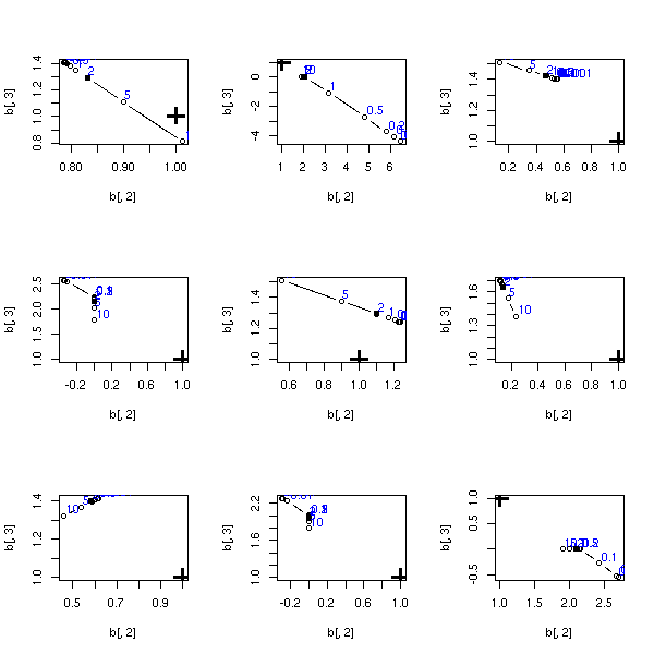
op <- par(mfrow=c(3,3))
for (i in 1:9) {
  my.lasso.test(1000)
}
par(op)
but there is already a function
library(help=lasso2)
library(lasso2)
?l1ce
?gl1ce
The same example.
%%G  BUG in lasso2
# There is not plot because of a bug in the "l1ce"
# function: first, it only accepts a data.frame;
# second. this data.frame has to be a global variable...

library(lasso2)
set.seed(73823)
#other.lasso.test <- function (n=20) {
  s <- .1
  x <- rnorm(n)
  x1 <- x + s*rnorm(n)
  x2 <- x + s*rnorm(n)
  y <- x1 + x2 + 1 + rnorm(n)
  d <- data.frame(y,x1,x2)
  lambda <- c(0, .001, .01, .1, .2, .5, 1, 2, 5, 10)
  b <- matrix(nr=length(lambda), nc=dim(d)[2])
  for (i in 1:length(lambda)) {
    try( b[i,] <- l1ce(y~x1+x2, data=d, bound=lambda[i], absolute.t=T)$coefficients )
    # I got the very informative error message:
    #   Oops, something went wrong in .C("lasso",..): -1
  }
  plot(b[,2], b[,3],
       type="b",
       xlim=range(c(b[,2],1)), ylim=range(c(b[,3],1)))
  text(b[,2], b[,3], lambda, adj=c(-.2,-.2), col="blue")
  points(1,1,pch="+", cex=3, lwd=3)
  points(b[8,2],b[8,3],pch=15)
#}
#other.lasso.test()
%--

op <- par(mfrow=c(3,3))
for (i in 1:9) {
  other.lasso.test()
}
par(op)
TODO:
y ~ x1 + x2
LS, ridge, lasso, PLS, PCR, best subset (leap): plot(b2~b1)
(some of these methods are discrete, others are continuous)
In particular, remark that ridge regression is very
similar to PLS ou PCR.
Let us start with ridge regression (red) and the lasso (black): the former seems better.
get.sample <- function (n=20,s=.1) {
  x <- rnorm(n)
  x1 <- x + s*rnorm(n)
  x2 <- x + s*rnorm(n)
  y <- x1 + x2 + 1 + rnorm(n)
  data.frame(y,x1,x2)
}
lambda <- c(0, .001, .01, .1, .2, .5, 1, 2, 5, 10)

do.it <- function (n=20,s=.1) {
  d <- get.sample(n,s)
  y <- d$y
  x <- cbind(d$x1,d$x2)
  ridge <- matrix(nr=length(lambda), nc=1+dim(x)[2])
  for (i in 1:length(lambda)) {
    ridge[i,] <- my.ridge(y,x,lambda[i])
  }
  lasso <- matrix(nr=length(lambda), nc=1+dim(x)[2])
  for (i in 1:length(lambda)) {
    lasso[i,] <- my.lasso(y,x,lambda[i])
  }
  xlim <- range(c( 1, ridge[,2], lasso[,2] ))
  ylim <- range(c( 1, ridge[,3], lasso[,3] ))
  plot(ridge[,2], ridge[,3],
       type = "b", col = 'red',
       xlim = xlim, ylim = ylim)
  points(ridge[8,2],ridge[8,3],pch=15,col='red')
  lines(lasso[,2], lasso[,3], type="b")
  points(lasso[8,2],lasso[8,3],pch=15)
  points(1,1,pch="+", cex=3, lwd=3)
}

op <- par(mfrow=c(3,3))
for (i in 1:9) {
  do.it()
}
par(op)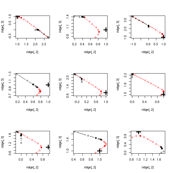
With larger samples, the lasso goes in the wrong direction...
op <- par(mfrow=c(3,3))
for (i in 1:9) {
  do.it(100)
}
par(op)
On the contrary, when there is little multicolinearity, both methods give similar results -- similarly bad results.
op <- par(mfrow=c(3,3))
for (i in 1:9) {
  do.it(20,10)
}
par(op)
Actually, Principal Component Regression (PCR) and Partial Least Squares (PLS) are discrete analogues of ridge regression. WE shall ofter prefer ridge regression, because the parameter can vary continuously.
my.pcr <- function (y,x,k) {
  n <- dim(x)[1]
  p <- dim(x)[2]
  ym <- mean(y)
  xm <- apply(x,2,mean)
  # Ideally, we should also normalize x and y...
  # (exercise left to the reader)
  y <- y - ym
  x <- t( t(x) - xm )
  pc <- princomp(x)
  b <- lm(y~pc$scores[,1:k]-1)$coef
  b <- c(b, rep(0,p-k))
  b <- pc$loadings %*% b
  names(b) <- colnames(x)
  b <- c(ym-t(b)%*%xm, b)
  b
}
get.sample <- function (n=20, s=.1) {
  x <- rnorm(n)
  x1 <- x + s*rnorm(n)
  x2 <- x + s*rnorm(n)
  x3 <- x + s*rnorm(n)
  x4 <- x + s*rnorm(n)
  x <- cbind(x1,x2,x3,x4)
  y <- x1 + x2 - x3 - x4 + 1 + rnorm(n)
  list(x=x,y=y)
}
pcr.test <- function (n=20, s=.1) {
  s <- get.sample(n,s)
  x <- s$x
  y <- s$y
  pcr <- matrix(nr=4,nc=5)
  for (k in 1:4) {
    pcr[k,] <- my.pcr(y,x,k)
  }
  plot(pcr[,2], pcr[,3],
       type = "b",
       xlim = range(c(pcr[,2],1)),
       ylim = range(c(pcr[,3],1)))
  points(pcr[4,2], pcr[4,3], lwd=2)
  points(1,1, pch="+", cex=3, lwd=3)
}
pcr.test()
TODO: add PLS

TODO: Put a title to the following section
(PCR/ridge regression comparison)
pcr.test <- function (n=20, s=.1) {
  s <- get.sample(n,s)
  x <- s$x
  y <- s$y

  lambda <- c(0, .001, .01, .1, .2, .5, 1, 2, 5, 10)
  ridge <- matrix(nr=length(lambda), nc=1+dim(x)[2])
  for (i in 1:length(lambda)) {
    ridge[i,] <- my.ridge(y,x,lambda[i])
  }

  pcr <- matrix(nr=4,nc=5)
  for (k in 1:4) {
    pcr[k,] <- my.pcr(y,x,k)
  }

  xlim <- range(c( 1, ridge[,2], pcr[,2] ))
  ylim <- range(c( 1, ridge[,3], pcr[,3] ))
  plot(ridge[,2], ridge[,3],
       type = "b", col = 'red',
       xlim = xlim, ylim = ylim)
  points(ridge[4,2], ridge[4,3],
         pch = 15, col = 'red')

  lines(pcr[,2], pcr[,3], type="b")
  points(pcr[4,2], pcr[4,3], lwd=2)
  points(1,1, pch="+", cex=3, lwd=3)
}
op <- par(mfrow=c(3,3))
for (i in 1:9) {
  pcr.test()
}
par(op)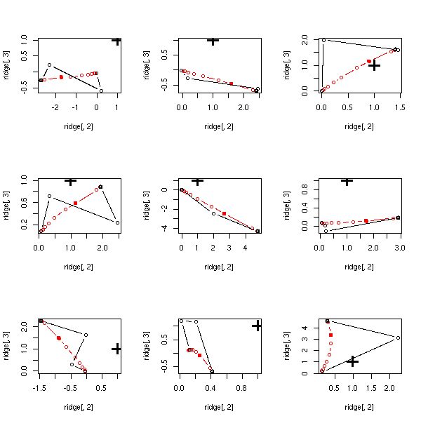
We have seen that ridge regression, lasso or splines couls be defined as optimization problems in which one tries to minimize a penalized sum of squares (a sum of squares, interpreted as a distance between the model forecasts and the actual values, as in Least Squares methods, to which we add a "penality" term, that grows with the complexity, the "naughtiness" of the model).
You can do the same thing with Maximum Likelihood Methods: the likelihood is a probability (usually, you do not consider the likelihood, which tends to be a product, but the log-likelihood, which tends to be a sum -- less unwieldy), to which you can add a penality for the model complexity.
TODO: Find examples (I have none...)

This work is licensed under a Creative Commons Attribution-NonCommercial-ShareAlike 2.5 License.
Vincent Zoonekynd
<zoonek@math.jussieu.fr>
latest modification on Sat Jan 6 10:28:21 GMT 2007