
Introduction to statistical tests: TODO: REWRITE THIS SECTION
The Zoo of statistical tests: Parametric Tests
The Zoo of Statistical Tests: discrete variables and the Chi^2 test
The Zoo of Statistical Tests: non-parametric tests
Estimators
TO SORT
TODO: give the structure of this chapter
motivation of statistical tests
notion of estimator, bias, MSE
...
MLE (should be in a section of its own)
Bayesian methods (in a section of their own)

(TODO)

TODO: list the more important tests (Student and Chi^2)
Student T test: compare a mean with a given number
                compare the mean in two samples
  There are generalizations for more than two samples
  (analysis of variance) and for non-gaussian samples
  (Wilcoxon).
  One can devise similar tests to compare the variance of
  a sample with a given number or to compare the variance
  of two samples.

Chi^2 test: to compare the distribution of a qualitative
  variable with predetermined values, to compare the
  distribution of a qualitative variable in two
  samples. One can also use it to check if two qualitative
  variables are independant. However, it is only an
  approximation, valid for large samples (more than 100
  observations, more that 10 observations per class).

TODO: check if we can do without the Chi^2 test:
  - binary variable:      bimom.test
  - multinomial test:     ???
  - Independance Chi^2:   fisher.test
  - two variables:        fisher.test
We want to answer a question of the kind "Does tobacco increase the risk of cancer?", "Does the proximity of a nuclear waste reprocessing plant increase the risk of leukemia?", "Is the mean of the population from which this sample was drawn zero, given that the sample mean is 0.02?"
Let us detail the problem "Have those two samples the same mean?" (it is a simplification of the problem "Do those two samples come from the same population?").
Let us consider a first population, on which is defined a statistical variable (with a gaussian distribution), from which we get a sample. We do the same for a second population, with the same population mean.
We can then consider the statistical variable
sample mean in the first sample - sample mean in the
second sample
and find its distribution.
If we measure a certain value of this difference, we can compute the probability of obtaining a difference at least as large.
If
P( difference > observed difference ) < alpha,
(for a given value of alpha, say 0.05), we reject the hypothesis "the two means are equal", with a risk equal to alpha.
But beware, this result is not certain at all. There can be two kinds of error: either wrongly clain that they are different (this happens with a probability alpha) or wrongly claim that the two means are equal.
Beware again, those tests are only valid under certain conditions (gaussian variables, same variance, etc.).
If we really wish to be rigorous, we do not consider a single hypothesis, but two: for instamce "the means are equal" and "the means are different"; or "the means are equal" and "the first mean is larger than the second". We would use the second formulation if we can a priori reject the fact that the first mean is lower than the second -- but this has to come from information independant from the samples at hand.
The statistical tests will never tell "the hypothesis is true": they will merely reject or fail to reject the hypothesis stating "there is nothing significant". (This is very similar to the development of science as explained by K. Popper: we never prove that something is true, we merely continuously try to prove it wrong and fail to do so.)
Let us consider two hypotheses: the null hypothesis H0, "there is no noticeable effect" (for instance, "tobacco does not increas the risk of cancer", the proximity of a waste recycling plant does not increas the risk of leukemia) and the alternative hypothesis H1, "there is a noticeable effect" (e.g., "tobacco increases the risk of cancer"). The alternative hypothesis can be symetric ("tobacco increases of decreases the risk of cancer") or not ("tobacco increases the risk of cancer"). To choose an asymetric hypothesis means that we reject, a priori, half of the hypothesis: it can be a prejudice, so you should think carefully before choosing an asymetric alternative hypothesis.
H0 is sometimes called the "conservative hypothesis", because it is the hypothesis we keep if the results of the test are not conclusive.
To wrongly reject the null hypothesis (i.e., to wrongly conclude "there is an effet" or "there is a noticeable difference").
For instance, if the variable X follows a gaussian distribution, we expect to get values "in the middle" of the bell-shaped curve. If we get extreme values, we shall reject, sometimes wrongly, the null hypothesis (that the mean is actually zero). The type I error corresponds to the red part in the following plot.
colorie <- function (x, y1, y2, N=1000, ...) {
  for (t in (0:N)/N) {
    lines(x, t*y1+(1-t)*y2, ...)
  }
}
# No, there is already a function to do this
colorie <- function (x, y1, y2, ...) {
  polygon( c(x, x[length(x):1]), c(y1, y2[length(y2):1]), ... )
}
x <- seq(-6,6, length=100)
y <- dnorm(x)
plot(y~x, type='l')
i = x<qnorm(.025)
colorie(x[i],y[i],rep(0,sum(i)) ,col='red')
i = x>qnorm(.975)
colorie(x[i],y[i],rep(0,sum(i)) ,col='red')
lines(y~x)
title(main="Type I error")
Probability (if the null hypothesis is true) to get a result at least as extreme. It is the probability of making a type I error.
Wrongly accepting the null hypothesis (i.e., wrongly concluding "there is no statistically significant effect" or "there is no difference").
In all rigour, it is not an error, because one never says "H0 is true" but "we do not reject H0 (yet)". It is not an error, but a missed opportunity.
The type II error is the area of the red part in the following plot. The middle bell-shaped curve is the distribution predicted by the null hypothesis, the other one is the actual distribution of the population.
x <- seq(-6,6, length=1000)
y <- dnorm(x)
plot(y~x, type='l')
y2 <- dnorm(x-.5)
lines(y2~x)
i <- x>qnorm(.025) & x<qnorm(.975)
colorie(x[i],y2[i],rep(0,sum(i)), col='red')
segments( qnorm(.025),0,qnorm(.025),dnorm(qnorm(.025)), col='red' )
segments( qnorm(.975),0,qnorm(.975),dnorm(qnorm(.975)), col='red' )
lines(y~x)
lines(y2~x)
title(main="High risk of type II error")

If the two curves are sufficiently far appart (i.e., if the difference of means is more significant), the risk is much lower.
x <- seq(-6,6, length=1000)
y <- dnorm(x)
plot(y~x, type='l')
y2 <- dnorm(x-3.5)
lines(y2~x)
i <- x>qnorm(.025) & x<qnorm(.975)
colorie(x[i],y2[i],rep(0,sum(i)), col='red')
segments( qnorm(.025),0,qnorm(.025),dnorm(qnorm(.025)), col='red' )
segments( qnorm(.975),0,qnorm(.975),dnorm(qnorm(.975)), col='red' )
lines(y~x)
lines(y2~x)
title(main="Lower risk of type II error")

You can plot the probability of type II error against the mean difference (contrary to the type I error, the risk of type II error is not a constant but depends on the actual value of the parameter: this is why this risk is often considered as difficult to compute and people tend to fail to mention it in elementary courses).
delta <- seq(-1.5, 1.5, length=500)
p <- NULL
for (d in delta) {
  p <- append(p,
              power.t.test(delta=abs(d), sd=1, sig.level=0.05, n=20,
                           type='one.sample')$power)
}
plot(1-p~delta, type='l',
     xlab='mean difference', ylab="propability of a type II error",
     main="type II error in a Student T test")
abline(h=0,lty=3)
abline(h=0.05,lty=3)
abline(v=0,lty=3)
The power of a test is
1 - P( type II error ).
Usually, the power is not a number but a function. The null hypothesis is often of the form H0: "mu = mu0" and the alternative hypothesis of the form H1: "mu different from mu0". The power will depend on the actual value of mu: if mu is close to mu0, the type II error probability is hygh and the power is low; on the contrary, if mu and mu0 are very different. the probability of type II error is lower and the power higher.
delta <- seq(0, 1.5, length=100)
p <- NULL
for (d in delta) {
  p <- append(p,
              power.t.test(delta=d, sd=1, sig.level=0.05, n=20,
                           type='one.sample')$power)
}
plot(p~delta, type='l',
     ylab='power', main='Power of a one-sample t-test')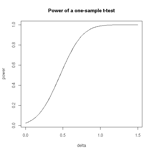
The power plays an important role when you design an experiment. Let us imagine that we want to know if the mean mu of a certain variable on a certain population equals mu0. We want to be able to detect a difference at least epsilon in at least 80% of the cases, with a type I error risk inferior to 5%: what should be the sample size?
In other words, we want that the power of the test H0: << mu = mu0 >> against H1: << abs(mu - mu0) > epsilon >> with a confidence level alpha=0.05 be at least 0.80 ("tradition" suggests a power equal to 0.80, and a confidence level 0.05).
The "power.t.test" performs those computations (for Student's T test).
> power.t.test(delta=.1, sd=1, sig.level=.05, power=.80, type='one.sample')

   One-sample t test power calculation

            n = 786.8109
        delta = 0.1
           sd = 1
    sig.level = 0.05
        power = 0.8
  alternative = two.sided
You can ask the question in any direction. For instance, the experiment has already been carried out, with a sample of size n: what is the minimal difference in mean we can expect to spot if we want the power of the test to be 0.08?
> power.t.test(n=100, sd=1, sig.level=.05, power=.80, type='one.sample')

   One-sample t test power calculation

            n = 100
        delta = 0.2829125
           sd = 1
    sig.level = 0.05
        power = 0.8
  alternative = two.sided
Here is a plot of this minimum noticeable difference against the sample size.
N <- seq(10,200, by=5)
delta <- NULL
for (n in N) {
  delta <- append(delta,
                  power.t.test(n=n, sd=1, sig.level=.05,
                               power=.80, type='one.sample')$delta
                 )
}
plot(delta~N, type='l', xlab='sample size')
delta <- NULL
for (n in N) {
  delta <- append(delta,
                  power.t.test(n=n, sd=1, sig.level=.01,
                               power=.80, type='one.sample')$delta
                 )
}
lines(delta~N, col='red')
delta <- NULL
for (n in N) {
  delta <- append(delta,
                  power.t.test(n=n, sd=1, sig.level=.001,
                               power=.80, type='one.sample')$delta
                 )
}
lines(delta~N, col='blue')
legend(par('usr')[2], par('usr')[4], xjust=1,
       c('significance level=.05', 'significance level=.01', 'significance level=.001'),
       col=c(par('fg'), 'red', 'blue'),
       lwd=1, lty=1)
title(main='Sample size and difference detected for tests of pover 0.80')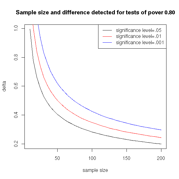
You might want to read:
http://www.stat.uiowa.edu/~rlenth/Power/2badHabits.pdf
http://www.stat.uiowa.edu/techrep/tr303.pdf
A hypothesis is said to be simple if it entails a complete knowledge of the distribution of the random variables. For instance, if we are looking for the mean of a gaussian variable of variance 1 (we already know the variance), the hypothesis H0: "the mean is zero" is simple. On the contrary, if we are looking for the mean of a gaussian variable (we know the variable is gaussian, but we do not know its variance -- we are not interested in it), this hypothesis is not simple.
Here is another example: we have a sample that comes either from a population 1 (described by a random variable of mean 3 and variance 2), or from a population 2 (described by a random variable of mean 1 and variance 1). In this case, both hypotheses H0: "the sample comes from population 1" and H1: "the sample comes from population 2" are simple.
A non-simple hypothesis.
Quite often, the alternative assumptions (H1) are composite: if H1 is true, we know that the distribution has a certain form, with a parameter that has not a certain value -- but we do not know its value.
Let us consider a random variable, whose distribution is not completely known: for instance, we know it is a gaussian distribution of variance 1, but the mean is unknown.
If we estimate this mean as a single number, we are sure to be wrong: the actual mean might be close to our proposal, but there is no reason it should be exactly this one, up to the umpteenth decimal. Instead, we can give a confidence interval -- note the use of an indefinite article: there are many such intervals (you can shift it to the left or to the right -- and doing so will change its width).
TODO: check that I give an example with several intervals.
Here are two interpretations of this notion of "confidence interval".
(1) It is an interval in which we have a 95% probability of finding the sample mean.
(2) More naively, it is an interval that has a 95% probability of containing the population mean (i.e., the actual mean).
Actually, these two interpretations are equivalent. As I was very dubious, let us check it on a simulation (here, I draw the population mean at random, and this prior distribution does not play any role).
TODO: say that it is bayesian...
# Sample size
n <- 100
# Number of points to draw the curve
N <- 1000
v <- vector()
for (i in 1:N) {
  m <- runif(1)
  x <- m+rnorm(n)
  int <- t.test(x)$conf.int
  v <- append(v, int[1]<m & m<int[2])
}
sum(v)/N
We get 0.95.
From this, we get two interpretations of the p-value: first, as the probability pf getting results at least as extre,e if H0 is true (this is the definition); second, it is the probability of being the in "the" confidence interval.
TODO: explain a bit more. I said that "the" confidence
interval was not uniquely defined, and thus, that we
should not use a definite article...
The p-value is NOT the probability that H0 be true. To convince yourself of this, consider gaussian random variable, of variance 1 and unknown mean. From a sample, we test H0: "the mean is 0" against H1: "the mean is not 0". We will get a certain p-value.
> n <- 10              # Sample size
> m <- rnorm(1)        # Unknown mean
> x <- m + rnorm(n)    # Sample
> t.test(x)$p.value    # p-value
[1] 0.2574325
But what is the probability that the mean be exactly zero? In our simulation, this probability is zero: the mean is almost surely non-zero.
> m
[1] 0.7263967
We would like to set the power of a test, in the same way we choose the level of confidence. But there is a problem: if H1 is not a simple hypothesis (i.e., if it is not a single hypothesis, as "mu=0" but a set of hypotheses, as "mu!=0", "mu>0" or "mu>1"), the power is not a number but a function, that depends on the simple hypotheses contained in H1.
A test is UMP (Uniformly Most Powerful) for a given confidence level alpha if, for any simple hypothesis in H1, it has the largest power among the tests with confidence level alpha.
Most of the time, statistical tests assume that the random variables studied are gaussian (and even, when there are several, that they have the same variance). Non-parametric tests do not make such assumptions -- xwe say that they are more "robust" -- but, as a counter part, they are less powerful.
Here are a few examples of parametric and non-parametric tests.
TODO: is it the right place for this list?
Aim                   Parametric tests             Non-parametric tests
----------------------------------------------------------------------------
compare two means     Student's T test             Wilcoxon's U test

compare more than     Anova (analysis of           Kruskal--Wallis test
two means             variance)

Compare two           Fisher's F test              Ansari-Bradley or
variances                                          Mood test

Comparing more than   Bartlett test                Fligner test
A (parametric) test is robust if its results are still valid when its assumptions are no longer satisfied (especially if the random variables studied are no longer gaussian).
A statistic (mean, median, variance, trimmed mean, etc.) is resistant if it does not depend much on extreme values. For instance, the mean is not resistant, while the median is: a single extreme value can drastically change the mean, while it will not change the median.
> x <- rnorm(10)
> mean(x)
[1] -0.08964153
> mean(c(x,10^10))      # We add an extreme value
[1] 909090909

> median(x)
[1] -0.2234618
> median(c(x,10^10))    # We add an extreme value
[1] -0.1949206
One can sometimes spot outliers with the Pearsons residuals:
sample density / density according to the model - 1
TODO: Example with circular data.
TODO
- Should you want them, there are statistical tests for the presence
  of outliers
- Outlier detection benchmark: use classical examples, such as
  library(robustbase)
  ?hkb
One should not try to automatically detect and remove the outliers: the first problem is that this is a multi-stage procedure (first the outlier detection and removal, then the rest of the analysis), whose performance should be assessed (the rest of the analysis will not perform as well as you think it should, because the data has been tampered with); the second problem is that the outlier removal is a black-and-white decision, either we keep the observation, or we remove it completely -- if we are unsure whether the observation is an actual outlier, we are sure to make mistakes.
Methods that remain efficient even in presence of outliers ("robust methods") do exist: use them!
The breaking point is the proportion of observations you can tamper with without being able to make the estimator arbitrarily "large".
This is a measure of robustness of an estimator.
For instance, the breaking point of the mean is zero: by changing a single observation, you can make the mean arbitrary large.
On the other hand, the breaking point of the median is 50%: if you change a single observation, the median will change, but its value vull be bounded by the rest of the cloud of points -- to make the median arbitrarily large, you would have to move (say) the top half of the data points.
The trimmed mean has a breaking point somewhere inbetween.
Location (mean): trimmed mean, median
Dispersion (standard deviation): IQR, MAD, Sn, L-moments, MCD

rlm, cov.rob
library(rrcov)
library(robustbase) (includes roblm)
1. We can look for a parameter of the distribution describing the population. If possible, we shall take an unbiased one, with the lowest variance possible. (However, we shall see later that certain biased estimators may be more interesting, because their mean square error is lower -- this is the case for ridge regression.)
2. Instead of a single value of this parameter, we can be looking for an interval containing it: we are then building a confidence interval.
3. We can also want to know if this parameter has (or not) a predefined value: we will then perform a test.
A p-value close to zero can mean two very different things: either the null hypothesis is very wrong, or ot is just slightly wrong but our sample is large enough to spot it. In the latter case, the difference between reality and the hypothesis is statistically significant, but for all practical purposes, it is negligible.
TODO: this problem with p-values is a starting point for the development
of bayesian methods.
http://www.stat.washington.edu/www/research/online/1994/bic.ps
Among all the possible tests, we want one for which the risks of type I and type II errors are as low as possible. Among the tests that can not be improved (i.e., we cannot modify them to get one with the same type I error risk and a lower type II error risk, and conversely), there is no means of choosing THE best. Indeed, we can plot those tests in the (type I error risk)x(type II error risk) plane: we get a curve. However, decision theory allows everyone to choose, among those tests, the one that becomes best one's taste taste for risk. One crude way of preceeding is to choose an upper bound on the type I error risk (alpha) and minimize the type II error risk.
For more details, read Simon's French book, "Decision Theory: an introduction to the mathematics of rationality", Ellis Horwood series in mathematics and its applications, Halsted Press, 1988.
Most R functions that perform (classical) tests are in the "stats" package (it is already loaded).
library(help="stats")
The list of functions is huge: look for those containing the "test" string.
> apropos(".test")
 [1] "ansari.test"          "bartlett.test"        "binom.test"
 [4] "Box.test"             "chisq.test"           "cor.test"
 [7] "fisher.test"          "fligner.test"         "friedman.test"
[10] "kruskal.test"         "ks.test"              "mantelhaen.test"
[13] "mcnemar.test"         "mood.test"            "oneway.test"
[16] "pairwise.prop.test"   "pairwise.t.test"      "pairwise.wilcox.test"
[19] "power.anova.test"     "power.prop.test"      "power.t.test"
[22] "PP.test"              "prop.test"            "prop.trend.test"
[25] "quade.test"           "shapiro.test"         "t.test"
[28] "var.test"             "wilcox.test"
One would expect those functions to yield a result as "Null hypothesis rejected" or "Null hypothesis not rejected" -- bad luck. The user has to know how to interpret the results, with a critical eye.
The result is mainly a number, the p-value. It is the probability to get a result at least as extreme. If it is close to one, we do not reject the hypothesis, i.e., the test did not find anything statistically significant; if it close to zero, we can reject the null hypothesis. More precisely, before performing the test, we choose a confidence level alpha (often 0.05; for human health, you will be more conservative an choose 0.01 or even less; if you want results with little data, if you do not mind that those results are not reliable, you can take 0.10): if p<alpha, you reject the null hypothesis, if p>alpha, you do not reject it.
Of course, you have to choose the confidence level alpha BEFORE performing the test (otherwise, you will choose it so that it produces the results you want)...
For instance,
> x <- rnorm(200)
> t.test(x)

      One Sample t-test

data:  x
t = 3.1091, df = 199, p-value = 0.002152
alternative hypothesis: true mean is not equal to 0
95 percent confidence interval:
 0.07855896 0.35102887
sample estimates:
mean of x
0.2147939
If we reject the null hypothesis (here: "the mean is zero"), we will be wrong with a probability 0.002152, i.e., in 2 cases out of 1,000.
We can check that with simulations: if the null hypothesis H0 is true, in 95% of the cases, we have p>0.05. Nore precisely, if H0 is true, the p-value is unifromly distributed in [0,1].
p <- c()
for (i in 1:1000) {
  x <- rnorm(200)
  p <- append(p, t.test(x)$p.value)
}
hist(p, col='light blue')
p <- sort(p)
p[950]
p[50]
x <- 1:1000
plot(p ~ x, main="p-value of a Student T test when H0 is true")

That was the type I error risk (wrongly rejecting the null hypothesis). Let us now focus on the type II error risk. This time, the population mean is non-zero. The risk will depend on the actual value of this mean -- but we do not know this value. If the mean is close to zero, the risk is high (we need a lot of data to spot small differences), if it is farther, the risk is lower.
# Sample size
n <- 10
# Number of simulations
# (sufficiently large to get a good approximation
# of the probability)
m <- 1000
# Number of points to draw the curve
k <- 50
# Maximum value for the actual mean
M <- 2
r <- vector()
for (j in M*(0:k)/k) {
  res <- 0
  for (i in 1:m) {
    x <- rnorm(10, mean=j)
    if( t.test(x)$p.value > .05 ){
      res <- res + 1
    }
  }
  r <- append(r, res/m)
}
rr <- M*(0:k)/k
plot(r~rr, type="l",
     xlab='difference in mean',
     ylab="type II error probability")

# Comparison with the curve produced by "power.t.test"
x <- seq(0,2,length=200)
y <- NULL
for (m in x) {
  y <- append(y, 1-power.t.test(delta=m, sd=1, n=10, sig.level=.05,
                                type='one.sample')$power)
}
lines(x,y,col='red')

# Theoretical curve
# (This is a Z test, not too different)
r2 <- function (p,q,conf,x) {
  p(q(1-conf/2)-x) - p(q(conf/2)-x)
}
f <- function(x) {
  p <- function (t) { pnorm(t, sd=1/sqrt(10)) }
  q <- function (t) { qnorm(t, sd=1/sqrt(10)) }
  r2(p,q,.05,x)
}
curve( f(x) , add=T, col="blue" )

# Theoretical curve (T test)
f <- function(x) {
  p <- function (t) { pt(sqrt(10)*t, 10) } # Is this correct?
  q <- function (t) { qt(t, 10)/sqrt(10) }
  r2(p,q,.05,x)
}
curve( f(x) , add=T, col="green" )

legend(par('usr')[2], par('usr')[4], xjust=1,
       c('simulation', 'power.t.test', '"exact" value, Z test',
         'excat value'),
       col=c(par('fg'),'red','blue','green'),
       lwd=1,lty=1)
title(main="Type II error risk in a Student T test")
We saw earlier that, if the null hypothesis is true, the p-values are uniformly distributed in [0,1]. Here is their distribution if H0 is false, for different values of the population mean.
N <- 10000
x <- 100*(1:N)/N
plot( x~I(x/100), type='n', ylab="cumulated percents", xlab="p-value" )
do.it <- function (m, col) {
  p <- c()
  for (i in 1:N) {
    x <- m+rnorm(200)
    p <- append(p, t.test(x)$p.value)
  }
  p <- sort(p)
  x <- 100*(1:N)/N
  lines(x ~ p, type='l', col=col)
}
do.it(0,   par('fg'))
do.it(.05, 'red')
do.it(.1,  'green')
do.it(.15, 'blue')
do.it(.2,  'orange')
abline(v=.05)
title(main='p-value distribution')
legend(par('usr')[2],par('usr')[3],xjust=1,yjust=1,
       c('m=0', 'm=0.05', 'm=.01', 'm=.015', 'm=.02'),
       col=c(par('fg'), 'red', 'green', 'blue', 'orange'),
       lty=1,lwd=1)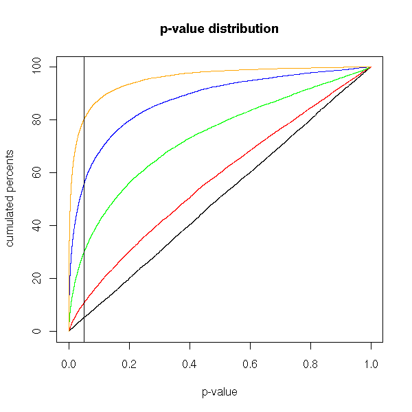
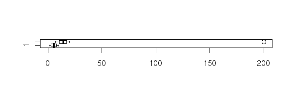
The manual gives this striking example, that explains why R does not give a clear result "Null hypothesis rejected" or "Null hypothesis not rejected". If we look at the data (with the eyes, on a plot -- always plot the data) we can state with little risk of error that the means are very different. However, the p-value is very high and suggests not to reject the null hypothesis that the means are equal. One problem is the size of the confidence interval: it is extremely large. Thus you should carefully look at the data. (On this example, there was one more problem: to perform a Student T test, the data have to be gaussian, to have the same variance, to be independant -- this is far from being the case).
TODO: somewhere in this document, state how to correctly
perform a test.
0. Choose a confidence level, a test
1. Plot the data
2. Check the assumptions. Change the test if needed.
3. Perform the test. Check the confidence interval.

TODO: where is my rant against T-values?

x <- 1:10
y <- c(7:20, 200)
boxplot(x,y, horizontal=T)
boxplot(x,y, log="x", horizontal=T)

> t.test(x, y)

      Welch Two Sample t-test

data:  x and y
t = -1.6329, df = 14.165, p-value = 0.1245
alternative hypothesis: true difference in means is not equal to 0
95 percent confidence interval:
 -47.242900   6.376233
sample estimates:
mean of x mean of y
  5.50000  25.93333
Of course, if we remove the outlier, 200, the result conforms with our intuition.
> t.test(1:10,y=c(7:20))

      Welch Two Sample t-test

data:  1:10 and c(7:20)
t = -5.4349, df = 21.982, p-value = 1.855e-05
alternative hypothesis: true difference in means is not equal to 0
95 percent confidence interval:
 -11.052802  -4.947198
sample estimates:
mean of x mean of y
      5.5      13.5
Similarly, if we use a non parametric test -- what we should have done from the very beginning.
> wilcox.test(x,y)

      Wilcoxon rank sum test with continuity correction

data:  x and y
W = 8, p-value = 0.0002229
alternative hypothesis: true mu is not equal to 0

Warning message:
Cannot compute exact p-value with ties in: wilcox.test.default(x, y)
Most of these tests are only valid for gaussian variables. Furthermore, if there are several samples, they often ask them to be independant and have the same variance.
Here, we want to find the mean of a random variable or, more precisely, to compare it with a predefined value.
?t.test
Assumptions: The variable is gaussian (if it is not, you can use Wilcoxon's U test).
We already gave an example above.
Here is the theory.
The null hypothesis is H0: "the mean is m", the alternative hypothesis is H1: "the mean is not m". We compute
              sample mean  -  m
T = ---------------------------------------
     sample standard deviation  /  sqrt(n)
(beware: there are two formulas for the standard deviation: the population standard deviation, with "n" in the denominator, and the sample standard deviation, with "n-1" -- R only uses the latter) (here, n is the sample size) and we reject H0 if
abs( T ) > t_{n-1} ^{-1} ( 1 - alpha/2 )where T_{n-1} is the student T distribution with n-1 degrees of freedom.
(With gaussian independant identically distributed random variables, T indeed follows this distribution -- you can actually define the Student T distribution that way.)
Here are a few Student T probability distribution functions. The larger n, the closer it is from a gaussian distribution.
curve(dnorm(x), from=-5, to=5, add=F, col="orange", lwd=3, lty=2)
curve(dt(x,100), from=-5, to=5, add=T, col=par('fg'))
curve(dt(x,5),  from=-5, to=5, add=T, col="red")
curve(dt(x,2),  from=-5, to=5, add=T, col="green")
curve(dt(x,1),  from=-5, to=5, add=T, col="blue")
legend(par('usr')[2], par('usr')[4], xjust=1,
       c('gaussian', 'df=100', 'df=5', 'df=2', 'df=1'),
       col=c('orange', par('fg'), 'red', 'green', 'blue'),
       lwd=c(3,1,1,1,1),
       lty=c(2,1,1,1,1))
title(main="Student's T probability distribution function")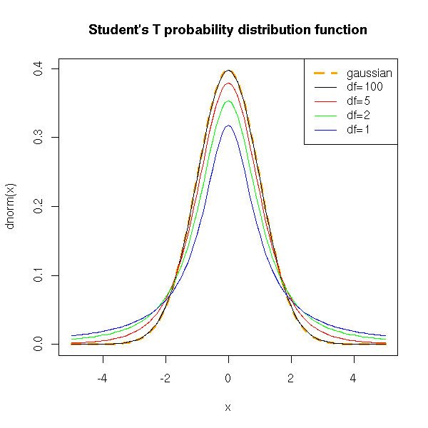
Let us now see how to use this, by hand.
We start with a sample from a gaussian population, whose mean we want to estimate.
> x <- rnorm(200)
> m <- mean(x)
> m
[1] 0.05875323
We now try to find an interval, centered on this sample mean, in which we ahve a 95% probability of finding the actual (population) mean (it is zero).
x <- rnorm(100)
n <- length(x)
m <- mean(x)
m
alpha <- .05
m + sd(x)/sqrt(n)*qt(alpha/2, df=n-1, lower.tail=T)
m + sd(x)/sqrt(n)*qt(alpha/2, df=n-1, lower.tail=F)
We get [m - 0.19, m + 0.19].
The "t.test" function provides a similar result.
> t.test(x, mu=0, conf.level=0.95)

      One Sample t-test

data:  x
t = 0.214, df = 99, p-value = 0.831
alternative hypothesis: true mean is not equal to 0
95 percent confidence interval:
 -0.1987368  0.2467923
sample estimates:
 mean of x
0.02402775
You can also experimentally check this with, with a simulation.
> m = c()
> for (i in 1:10000) {
+   m <- append(m, mean(rnorm(100)) )
+ }
> m <- sort(m)
> m[250]
[1] -0.1982188
> m[9750]
[1] 0.1999646
The interval is [-0.20, +0.20]: we get approximately the same result as the theoretical computations (this will always be the case with Monte-Carlo methods: the approximation is coarse, the convergence is slow, we need a lot of iterations to get a reliable result).
We can also plot the result of those simulations. We see that the actual mean is sometimes outside the confidence interval.
N <- 50
n <- 5
v <- matrix(c(0,0),nrow=2)
for (i in 1:N) {
  x <- rnorm(n)
  v <- cbind(v, t.test(x)$conf.int)
}
v <- v[,2:(N+1)]
plot(apply(v,2,mean), ylim=c(min(v),max(v)),
     ylab='Confidence interval', xlab='')
abline(0,0)
c <- apply(v,2,min)>0 | apply(v,2,max)<0
segments(1:N,v[1,],1:N,v[2,], col=c(par('fg'),'red')[c+1], lwd=3)
title(main="The population mean need not be in the confidence interval")
Let us perform a simulation to see what happens with non normal data -- a situation in which one should be using the Wilcoxon U test.
Let us first check with a distribution less dispersed that the gaussian one: the uniform distribution.
> N <- 1000
> n <- 3
> v <- vector()
> for (i in 1:N) {
    x <- runif(n, min=-1, max=1)
    v <- append(v, t.test(x)$p.value)
  }
> sum(v>.05)/N
[1] 0.932
Now with gaussian data.
> N <- 1000
> n <- 3
> v <- vector()
> for (i in 1:N) {
    x <- rnorm(n, sd=1/sqrt(3))
    v <- append(v, t.test(x)$p.value)
  }
> sum(v>.05)/N
[1] 0.952
Thus, the p-value is wrong when the variable is no longer gaussian: when we think we are rejecting the null hypothesis with a 5% risk of type I error, this risk is actually (for a uniform distribution, which is very far from pathological) 7%.
Let us seewhat happens to the confidence interval: we should be in it in 95% of the cases.
For a uniform distribution:
> N <- 1000
> n <- 3
> v <- vector()
> for (i in 1:N) {
    x <- runif(n, min=-1, max=1)
    r <- t.test(x)$conf.int
    v <- append(v, r[1]<0 & r[2]>0)
  }
> sum(v)/N
[1] 0.919
For a normal distribution:
> N <- 1000
> n <- 100
> v <- vector()
> for (i in 1:N) {
    x <- rnorm(n, sd=1/sqrt(3))
    r <- t.test(x)$conf.int
    v <- append(v, r[1]<0 & r[2]>0)
  }
> sum(v)/N
[1] 0.947
For the uniform distribution, we are in the confidence interval in 92% of the cases instead of the expected 95%. Actually, when the distribution is not gaussian, the results can be "wrong" in two ways: either the distribution is less dispersed than the gaussian, and the p-value is higher than stated by the test and the confidence interval provided is too small; or the distribution is more dispersed than the gaussian, the p-value will always be high, the confidence interval will be huge, and the test will no longer test anything (it loses its power, it will always state: there is nothing noticeable -- you can say it is blinded by the outliers).
TODO: I will say this later...
However, if the sample is much larger, the error becomes negligible.
> N <- 1000
> n <- 100
> v <- vector()
> for (i in 1:N) {
    x <- runif(n, min=-1, max=1)
    v <- append(v, t.test(x)$p.value)
  }
> sum(v>.05)/N
[1] 0.947

> N <- 1000
> n <- 100
> v <- vector()
> for (i in 1:N) {
    x <- runif(n, min=-1, max=1)
    r <- t.test(x)$conf.int
    v <- append(v, r[1]<0 & r[2]>0)
  }
> sum(v)/N
[1] 0.945
Let us now check the power of the test.
N <- 1000
n <- 10
delta <- .8
v <- vector()
w <- vector()
for (i in 1:N) {
  x <- delta+runif(n, min=-1, max=1)
  v <- append(v, t.test(x)$p.value)
  w <- append(w, wilcox.test(x)$p.value)
}
plot(sort(v), type='l', lwd=3, lty=2, ylab="p-valeur")
lines(sort(w), col='red')
legend(par('usr')[1], par('usr')[4], xjust=0,
       c('Student', 'Wilcoxon'),
       lwd=c(2,1),
       lty=c(2,1),
       col=c(par("fg"), 'red'))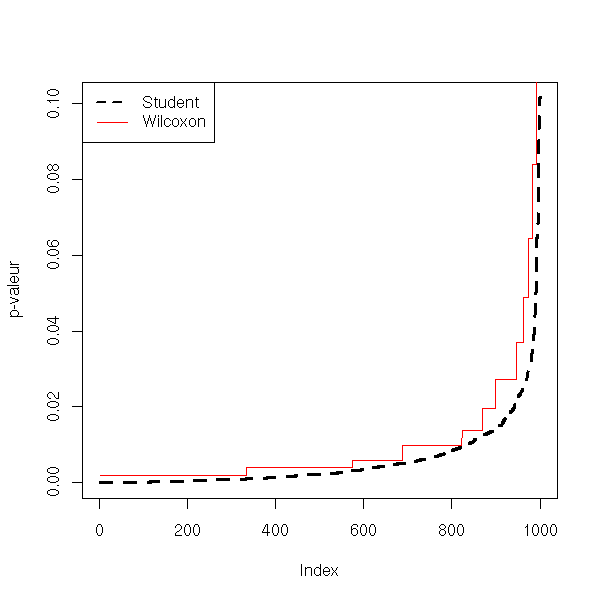
N <- 1000
n <- 100
delta <- .1
v <- vector()
w <- vector()
for (i in 1:N) {
  x <- delta+runif(n, min=-1, max=1)
  v <- append(v, t.test(x)$p.value)
  w <- append(w, wilcox.test(x)$p.value)
}
plot(sort(v), type='l', lwd=3, lty=2)
lines(sort(w), col='red')
legend(par('usr')[1], par('usr')[4], xjust=0,
       c('Student', 'Wilcoxon'),
       lwd=c(2,1),
       lty=c(2,1),
       col=c(par("fg"), 'red'))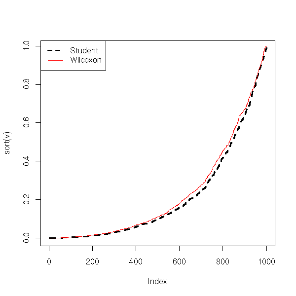
N <- 1000
n <- 100
delta <- .8
v <- vector()
w <- vector()
for (i in 1:N) {
  x <- delta+runif(n, min=-1, max=1)
  v <- append(v, t.test(x)$p.value)
  w <- append(w, wilcox.test(x)$p.value)
}
plot(sort(v), type='l', lwd=3, lty=2)
lines(sort(w), col='red')
legend(par('usr')[1], par('usr')[4], xjust=0,
       c('Student', 'Wilcoxon'),
       lwd=c(2,1),
       lty=c(2,1),
       col=c(par("fg"), 'red'))
From this, Student's T test seems robust: if the data are less dispersed than with a gaussian distribution, the p-value and the confidence interval are underestimated, but not too much. This effect disappeard if the sample is large enough.
But wait! Let us now see waht happens with a distribution more dispersed than the gaussian -- e.g., the Cauchy distribution.
> N <- 1000
> n <- 3
> v <- vector()
> for (i in 1:N) {
+   x <- rcauchy(n)
+   v <- append(v, t.test(x)$p.value)
+ }
> sum(v>.05)/N
[1] 0.974

> N <- 1000
> n <- 3
> v <- vector()
> for (i in 1:N) {
+   x <- rcauchy(n)
+   r <- t.test(x)$conf.int
+   v <- append(v, r[1]<0 & r[2]>0)
+ }
> sum(v)/N
[1] 0.988
The given confidence interval is too large: we are not in it in 95% of the cases, but much more. Things do not improve with an even larger sample.
> N <- 1000
> n <- 100
> v <- vector()
> for (i in 1:N) {
+   x <- rcauchy(n)
+   v <- append(v, t.test(x)$p.value)
+ }
> sum(v>.05)/N
[1] 0.982

> N <- 1000
> n <- 100
> v <- vector()
> for (i in 1:N) {
+   x <- rcauchy(n)
+   r <- t.test(x)$conf.int
+   v <- append(v, r[1]<0 & r[2]>0)
+ }
> sum(v)/N
[1] 0.986
Let us now check the test power: this is disastrous...
N <- 1000
n <- 10
delta <- 1
v <- vector()
w <- vector()
for (i in 1:N) {
  x <- delta+rcauchy(n)
  v <- append(v, t.test(x)$p.value)
  w <- append(w, wilcox.test(x)$p.value)
}
plot(sort(v), type='l', lwd=3, lty=2)
lines(sort(w), col='red')
N <- 1000
n <- 100
delta <- 1
v <- vector()
w <- vector()
for (i in 1:N) {
  x <- delta+rcauchy(n)
  v <- append(v, t.test(x)$p.value)
  w <- append(w, wilcox.test(x)$p.value)
}
plot(sort(v), type='l', lwd=3, lty=2)
lines(sort(w), col='red')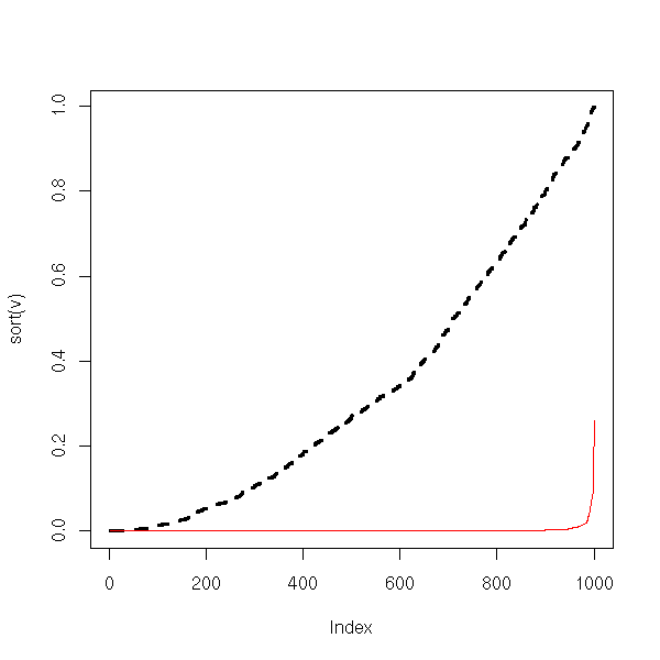
From this, we conclude that if the data are more dispersed than with a gaussian distribution, the power of the test decreases and nothing remains. Increasing th sample size does not improve things. In these situations, one should use non-parametric tests (or a parametric test adapted to the distribution at hand, or transform the data so that it looks more normal -- be beware, using the same data to choose the distribution or the trans formation and to perform the test will yield biased p-values).
> N <- 1000
> n <- 100
> v <- vector()
> w <- vector()
> for (i in 1:N) {
+   x <- rcauchy(n)
+   v <- append(v, t.test(x)$p.value)
+   w <- append(w, wilcox.test(x)$p.value)
+ }
> sum(v>.05)/N
[1] 0.976
> sum(w>.05)/N
[1] 0.948

> N <- 1000
> n <- 100
> v <- vector()
> w <- vector()
> for (i in 1:N) {
+   x <- 1+rcauchy(n)
+   v <- append(v, t.test(x)$p.value)
+   w <- append(w, wilcox.test(x)$p.value)
+ }
> sum(v<.05)/N
[1] 0.22
> sum(w<.05)/N
[1] 0.992
It is similar to the Student T test, but this time, we know the exact value of the variance: in this cas, the distribution of the test statistic is nolonger a Student T distribution but a gaussian distribution (often denoted Z).
In the real world, when we do not know the mean, we do not know the variance either -- thus, this test has little practical utility.
For large samples, Student's T distribution is well approximated by a gaussian distribution, so we can perform a Z test instead of a T test (that would be relevant if we we computing everything ourselves, but as the computer is there...)
We now consider two samples and we would like to know if they come from the same population. More simply, we would like to know if they have the same mean.
Here, we assume that the data are normal (do a qqplot or a Shapiro test), have the same variance (use an F test). If those conditions are not satisfied, you can use a Wilcoxon test.
We also assume that the variables are independant (this is not always the case: for instance, you might want to compare the length of the left and right humerus on a bunch of human skeletons; to get rid of the dependance problem, you can consider the length difference for each individual and compare it with zero.
For two samples of size n (it also works for samples of different sizes, but the formula is more complicated), one can show that the statistic
t = difference between the means / sqrt( (sum of the variances)/n )
follows a Student distribution with 2n-n degrees of freedom.
We shall reject the null hypothesis "the means are equal" if
abs(t) > abs( t(alpha, 2n-2) )
We could perform the test by hand, as above, but there is already a function to do so.
?t.test
> x <- rnorm(100)
> y <- rnorm(100)
> t.test(x,y)

      Welch Two Sample t-test

data:  x and y
t = -1.3393, df = 197.725, p-value = 0.182
alternative hypothesis: true difference in means is not equal to 0
95 percent confidence interval:
 -0.46324980  0.08851724
sample estimates:
  mean of x   mean of y
-0.03608115  0.15128514

> t.test(x, y, alternative="greater")

      Welch Two Sample t-test

data:  x and y
t = -1.3393, df = 197.725, p-value = 0.909
alternative hypothesis: true difference in means is greater than 0
95 percent confidence interval:
 -0.4185611        Inf
sample estimates:
  mean of x   mean of y
-0.03608115  0.15128514
Here is the example from the manual: the study of the efficiency of a soporific drug.
> ?sleep
> data(sleep)
> plot(extra ~ group, data = sleep)

> t.test(extra ~ group, data = sleep)
      Welch Two Sample t-test

data:  extra by group
t = -1.8608, df = 17.776, p-value = 0.0794
alternative hypothesis: true difference in means is not equal to 0
95 percent confidence interval:
 -3.3654832  0.2054832
sample estimates:
mean in group 1 mean in group 2
           0.75            2.33
Here, as the p-value is greater than 5%, we would conclude that the drug's effects are not noticeable in this sample. However, if you work for the drug's manufacturer, you would prefer a different conclusion. You can get it if you change the alternative hypothsis, that becomes H1: "the drug increases the time of sleep". (If you are honest, you choose the null and alternative hypotheses before performing the experiment, and this choice must be backed by prior data or knowledge: remarking that in this very experiment the sample mean is greater is not sufficient.)
> t.test(extra ~ group, data = sleep, alternative="less")

      Welch Two Sample t-test

data:  extra by group
t = -1.8608, df = 17.776, p-value = 0.0397
alternative hypothesis: true difference in means is less than 0
95 percent confidence interval:
       -Inf -0.1066185
sample estimates:
mean in group 1 mean in group 2
           0.75            2.33
TODO: There should be a section "How to lie with statistics"
1. Reusing the same data several times to increase the
   statistical significance of an effect.  (examples:
   choose H1 after looking at the data, use the data to
   choose the transformation to apply, etc.)
2. Using a statistical test whose asumptions are not
   satisfied (it can either yield more significant results
   or less significant results: e.g., if the test assumes
   that ******************** (deleted?)
3. Perform the same experiment several times and only
   publish the results that go in the direction you
   want. (Adverts by tobacco companies claiming that
   passive smoking is harmless are done that way.)
4. Misleading plots
   Adding a lot of unnecessary details
   3D effects
     - The most striking is the 3-dimensional piechart,
       with the part of interest at the forefront, so that
       it be deformed and larger)
     - You can also plot a quantity as a sphere (ar any
       3-dimensional object) of different scales: for a
       quantity twice as large, you can multiply all the
       dimensions by 2, thereby getting a volume eight
       times as large.
If you have more than two samples, you can perform an ANalysis Of VAriance (Anova). If you have two non-gaussain samples, you can perform a Wilcoxon U test. If you have more that two non-gaussian samples, you can turn to non-parametric analysis of variance with the Kruskal--Wallis test.
To compare means with a Student T test, we assume that: the samples are gaussian, independant and have the same variance.
Let us check what happens with gaussian non-equivariant samples.
TODO: check that there is no confusion between the Student T test and Welch's test (var.equal=T for the first, var.equal=F (the default) for the second).
N <- 1000
n <- 10
v <- 100
a <- NULL
b <- NULL
for (i in 1:N) {
  x <- rnorm(n)
  y <- rnorm(n, 0, v)
  a <- append(a, t.test(x,y)$p.value)
  b <- append(b, t.test(x/var(x), y/var(y))$p.value)
}
plot(sort(a), type='l', col="green")
points(sort(b), type="l", col="red")
abline(0,1/N)
And for the power:
N <- 1000
n <- 10
v <- 100
a <- NULL
b <- NULL
c <- NULL
d <- NULL
for (i in 1:N) {
  x <- rnorm(n)
  y <- rnorm(n, 100, v)
  a <- append(a, t.test(x,y)$p.value)
  b <- append(b, t.test(x/var(x), y/var(y))$p.value)
  c <- append(c, t.test(x, y/10000)$p.value)
  d <- append(d, wilcox.test(x, y)$p.value)
}
plot(sort(a), type='l', col="green")
points(sort(b), type="l", col="red")
points(sort(c), type="l", col="blue")
points(sort(d), type="l", col="orange")
abline(0,1/N)
legend(par('usr')[1], par('usr')[4],
       c('Student Test', 'Renormalized Student Test',
         'Student Test renormalized with the sample variances',
         "(Non-Parametric) Wilcoxson's U Test"),
       col=c('green', 'blue', 'red', 'orange'),
       lwd=1,lty=1)
title(main="Student's T test on non-equivariant samples")
With non-equivariant samples, the p-value of the Student test remains correct, but the power dramatically decreases. If the data look gaussian but have different variances, you had better normalize them andto perform a Student T test than perform a non-parametric test.
TODO: What about the Welch test???
There are several ways of comparing two means.
data(sleep)
boxplot(extra ~ group, data=sleep,
        horizontal=T,
        xlab='extra', ylab='group')
With a Student T test, if the data are gaussian (or a Welch test, if they are gaussian but have different variances).
> t.test(extra ~ group, data=sleep)

      Welch Two Sample t-test

data:  extra by group
t = -1.8608, df = 17.776, p-value = 0.0794
alternative hypothesis: true difference in means is not equal to 0
95 percent confidence interval:
 -3.3654832  0.2054832
sample estimates:
mean in group 1 mean in group 2
           0.75            2.33

> t.test(extra ~ group, data=sleep, var.equal=T)

        Two Sample t-test

data:  extra by group
t = -1.8608, df = 18, p-value = 0.07919
alternative hypothesis: true difference in means is not equal to 0
95 percent confidence interval:
 -3.3638740  0.2038740
sample estimates:
mean in group 1 mean in group 2
           0.75            2.33
With a Wilcoxon test, if we do not know that the data are gaussian, or if we suspect they are not (from a Shapiro--Wilk test, for instance).
> wilcox.test(extra ~ group, data=sleep)

      Wilcoxon rank sum test with continuity correction

data:  extra by group
W = 25.5, p-value = 0.06933
alternative hypothesis: true mu is not equal to 0

Warning message:
Cannot compute exact p-value with ties in: wilcox.test.default(x = c(0.7, -1.6,
With an analysis of variance (we will present this later -- with only two samples, it yields exactly the same result as the Student T test).
> anova(lm(extra ~ group, data=sleep))
Analysis of Variance Table

Response: extra
          Df Sum Sq Mean Sq F value  Pr(>F)
group      1 12.482  12.482  3.4626 0.07919 .
Residuals 18 64.886   3.605
---
Signif. codes:  0 `***' 0.001 `**' 0.01 `*' 0.05 `.' 0.1 ` ' 1
With a non parametric analysis of variance, i.e., a Kruskal--Wallis test.
> kruskal.test(extra ~ group, data=sleep)

      Kruskal-Wallis rank sum test

data:  extra by group
Kruskal-Wallis chi-squared = 3.4378, df = 1, p-value = 0.06372
Here are the results
Method                 p-value

Welch test             0.07919
Student T test         0.0794
Wilcoxon               0.06933
Analysis of Variance   0.07919
Kruskal--Wallis Test   0.06372
We are looking for the variance of a sample (whose mean is unknown).
Here is the theory.
The null hypothesis is H0: "the (population) variance is v", the alternative hypothesis is H1: "the variance is not v". We compute the statistic
Chi2 = (n-1) * (sample variance) / v
and je reject the null hypothesis H0 if
  Chi2 > Chi2_{n-1} ^{-1} ( 1 - alpha/2 )
or
  Chi2 < Chi2_{n-1} ^{-1} ( alpha/2 )
where Chi2_{n-1} is the Chi2 distribution with n-1 degrees of freedom.
Here is the Chi^2 probability distribution function, with various degrees of freedom.
curve(dchisq(x,2),  from=0, to=5, add=F, col="red",
      ylab="dchisq(x,i)")
n <- 10
col <- rainbow(n)
for (i in 1:n) {
  curve(dchisq(x,i),  from=0, to=5, add=T, col=col[i])
}
legend(par('usr')[2], par('usr')[4], xjust=1,
        paste('df =',1:n),
       lwd=1,
       lty=1,
       col=col)
title(main="Chi^2 Probability Distribution Function")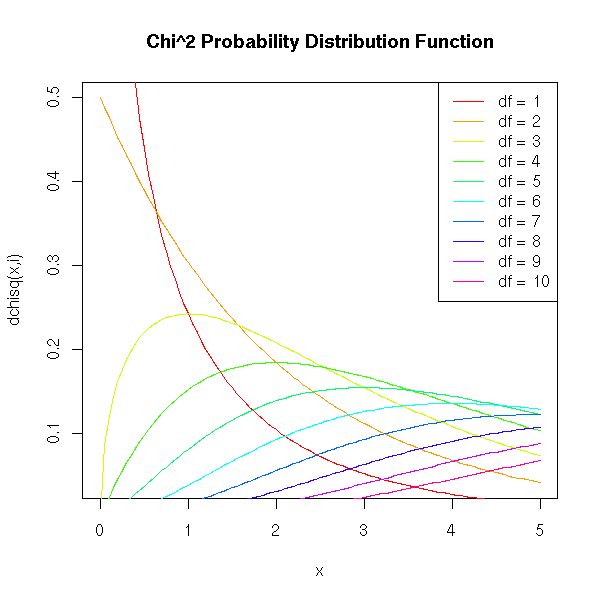
We can get a confidence interval for the standard deviation, by hand, as follows.
alpha <- .05
x <- rnorm(200)
n <- length(x)
v = var(x)
sd(x)
sqrt( (n-1)*v / qchisq(alpha/2, df=n-1, lower.tail=F) )
sqrt( (n-1)*v / qchisq(alpha/2, df=n-1, lower.tail=T) )
We get [0.91, 1.11].
We can check this with a simulation:
v <- c(0)
for (i in 1:10000) {
  v <- append(v, var(rnorm(200)) )
}
v <- sort(v)
sqrt(v[250])
sqrt(v[9750])
We get [0.90, 1.10].
With smaller samples, the estimation is less reliable: the confidence interval is larger, [0.68, 1.32].
v <- c(0)
for (i in 1:10000) {
  v <- append(v, var(rnorm(20)) )
}
v <- sort(v)
sqrt(v[250])
sqrt(v[9750])
I have not found an R function that performs those computations (the "var.test" works with two samples): we can write our own.
chisq.var.test <- function (x, var=1, conf.level=.95,
                            alternative='two.sided') {
  result <- list()
  alpha <- 1-conf.level
  n <- length(x)
  v <- var(x)
  result$var <- v
  result$sd <- sd(x)
  chi2 <- (n-1)*v/var
  result$chi2 <- chi2
  p <- pchisq(chi2,n-1)
  if( alternative == 'less' ) {
    stop("Not implemented yet")
  } else if (alternative == 'greater') {
    stop("Not implemented yet")
  } else if (alternative == 'two.sided') {
    if(p>.5)
      p <- 1-p
    p <- 2*p
    result$p.value <- p
    result$conf.int.var <- c(
      (n-1)*v / qchisq(alpha/2, df=n-1, lower.tail=F),
      (n-1)*v / qchisq(alpha/2, df=n-1, lower.tail=T),
    )
  }
  result$conf.int.sd <- sqrt( result$conf.int.var )
  result
}
x <- rnorm(100)
chisq.var.test(x)

# We can check tha the results are correct by looking at
# the distribution of the p-values: it should be uniform
# in [0,1].
v <- NULL
for (i in 1:1000) {
  v <- append(v, chisq.var.test(rnorm(100))$p.value)
}
plot(sort(v))
We can also compare the results with those of the "var.test" function, that works woth two samples. Either graphically,
p1 <- NULL
p2 <- NULL
for (i in 1:100) {
  x <- rnorm(10)
  p1 <- append(p1, chisq.var.test(x)$p.value)
  p2 <- append(p2, var.test(x, rnorm(10000))$p.value)
}
plot( p1 ~ p2 )
abline(0,1,col='red')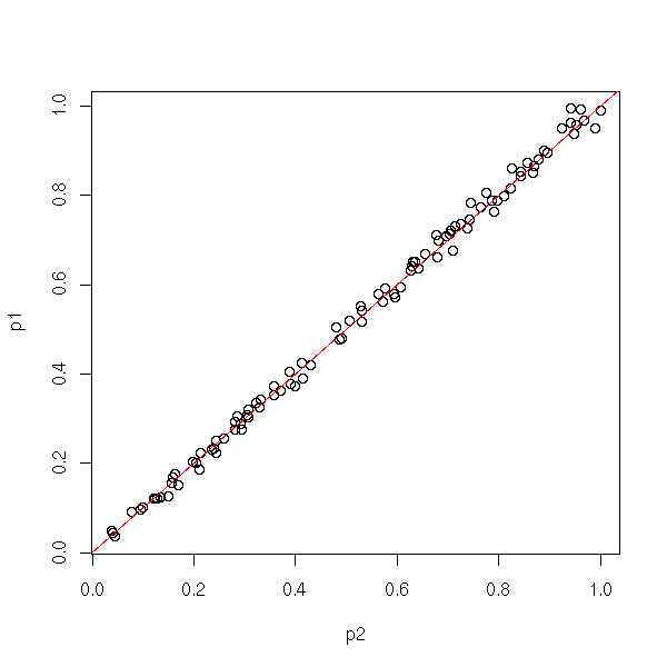
or with a computation (we shall see later what it means: this is a test on a regression, that tells us that p1=p2 with a p-value equal to 0.325).
> summary(lm(p1-p2~0+p2))

Call:
lm(formula = p1 - p2 ~ 0 + p2)

Residuals:
      Min        1Q    Median        3Q       Max
-0.043113 -0.007930  0.001312  0.009386  0.048491

Coefficients:
    Estimate Std. Error t value Pr(>|t|)
p2 -0.002609   0.002638  -0.989    0.325

Residual standard error: 0.01552 on 99 degrees of freedom
Multiple R-Squared: 0.009787,   Adjusted R-squared: -0.0002151
F-statistic: 0.9785 on 1 and 99 DF,  p-value: 0.325
Here, we want to know if two samples come from populations from the same variance (we are not interested in the mean).
We proceed as for the comparison of means, but instead of considering the difference of means, we consider the quotient of variances.
One will use such a test before a Student T test (to compare the mean in two samples), to check that the equivariance assumption is valid.
Here is the example with which we had illustrated the Student T test: indeed, the variances do not seem too different.
?var.test
> var.test( sleep[,1] [sleep[,2]==1], sleep[,1] [sleep[,2]==2] )

      F test to compare two variances

data:  sleep[, 1][sleep[, 2] == 1] and sleep[, 1][sleep[, 2] == 2]
F = 0.7983, num df = 9, denom df = 9, p-value = 0.7427
alternative hypothesis: true ratio of variances is not equal to 1
95 percent confidence interval:
 0.198297 3.214123
sample estimates:
ratio of variances
         0.7983426
Here is the theory behind this test.
The null hypothesis is H0: "the two populations have the same variance", the alternative hypothesis is H1: "the two populations do not have the same variance". We compute the statistic
     variance of the first sample
F = -------------------------------
     variance of the second sample
(here, I assume that the two samples have the same size, otherwise the formula becomes more complicated) and we reject H0 if
  F < F _{n1-1, n2-2} ^{-1} ( alpha/2 )
or
  F > F _{n1-1, n2-2} ^{-1} ( 1 - alpha/2 )
where F is Fisher's distribution.
Practically, we compute the quotient of variances with the largest variance in the numerator and we reject the null hypothesis that the variances are equal if
F > F(alpha/2, n1-1, n2-1)
where n1 and n2 are the sample sizes.
Here is an example, where the computations were performed by hand.
> x <- rnorm(100, 0, 1)
> y <- rnorm(100, 0, 2)
> f <- var(y)/var(x)
> f
[1] 5.232247
> qf(alpha/2, 99, 99)
[1] 0.6728417
> f > qf(alpha/2, 99, 99)
[1] TRUE
If we have more than two samples, we can use Bartlett's test. Of we have two non-gaussian samples, we can use Ansari's or Mood's non parametric test. Of there are more that two non-gaussian samples, we can use Fligner's test.
?bartlett.test
?ansari.test
?mood.test
?fligner.test
In a sample of 100 butterflies, we found 45 males and 55 females. Can we conclude that there are, in general, more males than females?
The number of female butterflies in a samples if 100 animals follows a binimial distribution B(100,p) and we want to test the null hypothesis H0: "p=0.5" against the alternative hypothesis H1: "p different from 0.5".
> binom.test(55, 100, .5)

      Exact binomial test

data:  55 and 100
number of successes = 55, number of trials = 100, p-value = 0.3682
alternative hypothesis: true probability of success is not equal to 0.5
95 percent confidence interval:
 0.4472802 0.6496798
sample estimates:
probability of success
                  0.55
In this example, the difference is not statistically significant.
If we were doing the computations by hand, we would not use the binomial test, but an approximation, with the "prop.test". But as the computer performscarries out the computations for us, we need not use it.
p <- .3
col.values <- c(par('fg'),'red', 'blue', 'green', 'orange')
n.values <- c(5,10,20,50,100)
plot(0, type='n', xlim=c(0,1), ylim=c(0,1), xlab='exact', ylab='approximate')
for (i in 1:length(n.values)) {
  n <- n.values[i]
  x <- NULL
  y <- NULL
  for (a in 0:n) {
    x <- append(x, binom.test(a,n,p)$p.value)
    y <- append(y, prop.test(a,n,p)$p.value)
  }
  o <- order(x)
  lines(x[o],y[o], col=col.values[i])
}
legend(par('usr')[1],par('usr')[4],
       as.character(n.values),
       col=col.values,
       lwd=1,lty=1)
title(main="Comparing the binomial test and its approximation")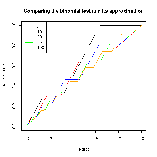
We can also compare the distribution of p-values of these two tests.
p <- .3
n <- 5
N <- 1000
e <- rbinom(N, n, p)
x <- y <- NULL
for (a in e) {
  x <- append(x, binom.test(a,n,p)$p.value)
  y <- append(y, prop.test(a,n,p)$p.value)
}
x <- sort(x)
y <- sort(y)
plot(x, type='l', lwd=3, ylab='p-value')
lines(y, col='red')
legend(par('usr')[2], par('usr')[3], xjust=1, yjust=0,
       c('exact', 'approximation'),
       lwd=c(3,1),
       lty=1,
       col=c(par("fg"),'red'))
title(main="Binomial test (H0 true)")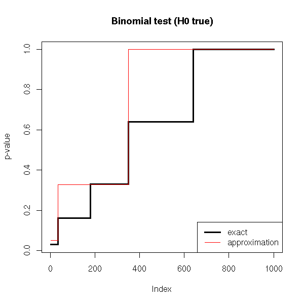
p1 <- .3
p2 <- .5
n <- 5
N <- 1000
e <- rbinom(N, n, p1)
x <- y <- NULL
for (a in e) {
  x <- append(x, binom.test(a,n,p2)$p.value)
  y <- append(y, prop.test(a,n,p2)$p.value)
}
x <- sort(x)
y <- sort(y)
plot(x, type='l', lwd=3, ylab='p-value')
lines(y, col='red')
legend(par('usr')[2], par('usr')[3], xjust=1, yjust=0,
       c('exact', 'approximation'),
       lwd=c(3,1),
       lty=1,
       col=c(par("fg"),'red'))
title(main="Binomial test (H0 false)")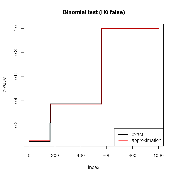
We remark that if H0 is true, the p-value is over-estimated (the test is too conservative, it is less powerful, it does not see anything significant while there is), but the wronger H0, the better the approximation.
TODO: alternative to the binomial test:
  glm(y~x, family=binomial)   # Logistic regression
(well, for p=0.5)

Question: and for p != 0.5?
You can do the same for multilogistic regression
The binomial test is fine, but it does not generalize: it allows you to study a binary variable, nothing more. But sometimes we need a comparable test to study qualitative variables with more than 2 values or to study several qualitative variables. There is no such "exact multinomial test" (you can devise one, but you would have to implement it...): instead, one uses the approximate Chi2 test.
The Chi2 test is a non parametric , non-rigorous (it is an approximation) test to compare distributions of qualitative variables. In spite of that, it is the most important discrete test.
One can show that if (X1, X2, ..., Xr) is a multinomial random variable, then
         ( X_1 - n p_1 )^2           ( X_r - n p_r )^2
Chi^2 = ------------------- + ... + --------------------
              n p_1                        n p_r
asymptotically follows a Chi^2 distribution with r-1 degrees of freedom. This tis is just an asymptotic result, that is sufficiently true if
n >= 100     (the sample is large enough)
n p_i >= 10  (the theoretical frequencies (counts) are not too small)
In particular, we get another mock binomial test.
p <- .3
col.values <- c(par('fg'),'red', 'blue', 'green', 'orange')
n.values <- c(5,10,20,50,100)
plot(0, type='n', xlim=c(0,1), ylim=c(0,1), xlab='exact', ylab='approximate')
for (i in 1:length(n.values)) {
  n <- n.values[i]
  x <- NULL
  y <- NULL
  z <- NULL
  for (a in 0:n) {
    x <- append(x, binom.test(a,n,p)$p.value)
    y <- append(y, chisq.test(c(a,n-a),p=c(p,1-p))$p.value)
    z <- append(z, prop.test(a,n,p)$p.value)
  }
  o <- order(x)
  lines(x[o],y[o], col=col.values[i])
  lines(x[o],z[o], col=col.values[i], lty=3)
}
legend(par('usr')[1],par('usr')[4],
       as.character(c(n.values, "prop.test", "chisq.test")),
       col=c(col.values, par('fg'), par('fg')),
       lwd=1,
       lty=c(rep(1,length(n.values)), 1,3)
      )
title(main="The binomial test and its approximations")
Or a mock multinomial test: let us check, with a simulation, that the p-values are close.
# A Monte Carlo multinomial test
multinom.test <- function (x, p, N=1000) {
  n <- sum(x)
  m <- length(x)
  chi2 <- sum( (x-n*p)^2/(n*p) )
  v <- NULL
  for (i in 1:N) {
    x <- table(factor(sample(1:m, n, replace=T, prob=p), levels=1:m))
    v <- append(v, sum( (x-n*p)^2/(n*p) ))
  }
  sum(v>=chi2)/N
}
multinom.test( c(25,40,25,25), p=c(.25,.25,.25,.25) )   # 0.13
chisq.test(    c(25,40,25,25), p=c(.25,.25,.25,.25) )   # 0.12

N <- 100
m <- 4
n <- 10
p <- c(.25,.25,.1,.4)
x <- NULL
y <- NULL
for (i in 1:N) {
  a <- table( factor(sample(1:m, n, replace=T, prob=p), levels=1:m) )
  x <- append(x, multinom.test(a,p))
  y <- append(y, chisq.test(a,p=p)$p.value)
}
plot(y~x)
abline(0,1,col='red')
title("Monte Carlo Multinomial Test and Chi^2 Test")
Here is the distribution of the p-values of a Chi^2 test.
# We sample 10 subjects in a 4-class population.
# We repeat the experiment 100 times.
N <- 1000
m <- 4
n <- 10
p <- c(.24,.26,.1,.4)
p.valeur.chi2 <- rep(NA,N)
for (i in 1:N) {
  echantillon <- table(factor(sample(1:m, replace=T, prob=p), levels=1:m))
  p.valeur.chi2[i] <- chisq.test(echantillon,p=p)$p.value
}
plot( sort(p.valeur.chi2), type='l', lwd=3 )
abline(0, 1/N, lty=3, col='red', lwd=3)
title(main="p-values in a Chi^2 test")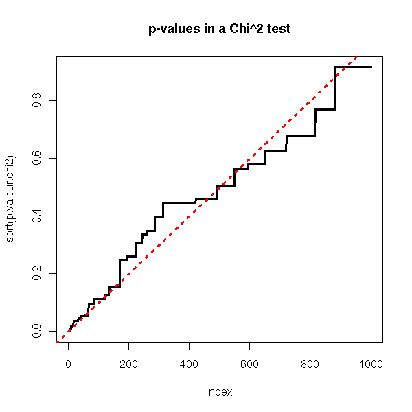
Let us consider the following situation: we measure two qualitative variables each with two values on a sample. In the whole population, the four classes occur with proportions 10%, 20%, 60%, 10%.
       A    B   total
C     10   20   30
D     60   10   70
total 70   30   100
We can get a sample as follows.
TODO: this code is ugly...

foo <- function (N) {
  population1 <- c(rep('A',10), rep('B',20), rep('A',60), rep('B',10))
  population1 <- factor(population1, levels=c('A','B'))
  population2 <- c(rep('C',10), rep('C',20), rep('D',60), rep('D',10))
  population2 <- factor(population2, levels=c('C','D'))
  o <- sample(1:100, N, replace=T)
  table( population2[o], population1[o] )
}
a <- foo(1000)
op <- par(mfcol=c(1,2))
plot( a, shade=T )
plot( t(a), shade=T )
par(op)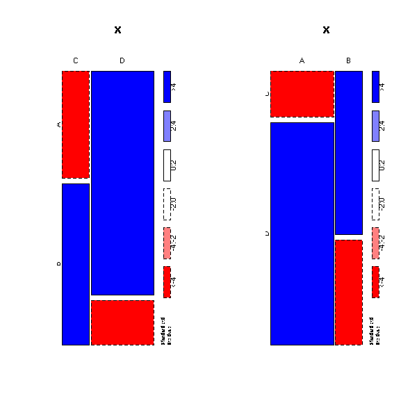
We would like to know wether these variables are independant or not. To do so, we take a sample (as always, we do not know the population direclty, we only know it through samples -- so we are not supposed to know the proportions I mentionned above); we compute the marginal proportions (i.e., the "total" row and column); the product of this row and column, so as to get the proportions one would observe if the variables were independant; we can then compare those proportions with the observed ones.
> n <- 100
> a <- foo(n)
> a/n
       A    B
  C 0.09 0.15
  D 0.65 0.11
> a1 <- apply(a/n,2,sum) # The "total" row
> a1
   A    B
0.74 0.26
> a2 <- apply(a/n,1,sum) # The "total" column
> a2
   C    D
0.24 0.76
> b <- a1 %*% t(a2)
> b
            C      D
  [1,] 0.1776 0.5624
  [2,] 0.0624 0.1976
> chisq.test(as.vector(a),p=as.vector(b))

      Chi-squared test for given probabilities

data:  as.vector(a)
X-squared = 591.7683, df = 3, p-value = < 2.2e-16

TODO
I think the syntax is different
chisq.test(rbind(as.vector(a), as.vector(b)))
Is the result the same?

TODO
Remark
One can also use the Chi^2 for a homogeneity test, i.e.,
to check if two samples come from the same population.
It IS an independance Chi^2 (independance between the
variable and the sample number): the syntax is the same.
chisq.test(rbind(as.vector(a), as.vector(b)))
Here, we want to check if two variables, given by a contingency table, are independant. It sounds like the Chi^2 test, but this time, it is an exact test, not an approximation.
Let us take the example we had examined above with the Chi^2 test.
> a
     A  B
  C  9 15
  D 65 11
> fisher.test(a)

      Fisher's Exact Test for Count Data

data:  a
p-value = 1.178e-05
alternative hypothesis: true odds ratio is not equal to 1
95 percent confidence interval:
 0.03127954 0.32486526
sample estimates:
odds ratio
 0.1048422
With a smaller sample, it is less clear.
> fisher.test( foo(10) )

      Fisher's Exact Test for Count Data

data:  foo(10)
p-value = 1
alternative hypothesis: true odds ratio is not equal to 1
95 percent confidence interval:
  0.003660373 39.142615141
sample estimates:
odds ratio
 0.3779644

n1 <- 10
n2 <- 100
N <- 1000
x1 <- rep(NA,N)
x2 <- rep(NA,N)
for (i in 1:N) {
  x1[i] <- fisher.test(foo(n1))$p.value
  x2[i] <- fisher.test(foo(n2))$p.value
}
plot( sort(x1), type='l', lwd=3, ylab='p-valeur')
lines( sort(x2), col='blue', lwd=3 )
abline(0,1/N,col='red',lwd=3,lty=3)
abline(h=c(0,.05),lty=3)
abline(v=c(0,N*.05),lty=3)
title(main="p-value of a Fisher test, H0 false")
legend(par('usr')[1],par('usr')[4],
       c("n=10", "n=100"),
       col=c(par('fg'), 'blue'),
       lwd=3,
       lty=1)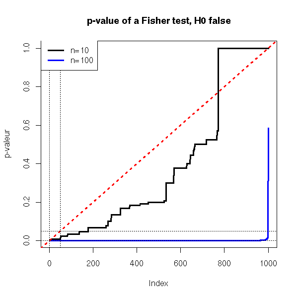
foo <- function (N) {
  population1 <- c(rep('A',2), rep('B',8), rep('A',18), rep('B',72))
  population1 <- factor(population1, levels=c('A','B'))
  population2 <- c(rep('C',2), rep('C',8), rep('D',18), rep('D',72))
  population2 <- factor(population2, levels=c('C','D'))
  o <- sample(1:100, N, replace=T)
  table( population2[o], population1[o] )
}
n1 <- 10
n2 <- 100
N <- 1000
x1 <- rep(NA,N)
x2 <- rep(NA,N)
for (i in 1:N) {
  x1[i] <- fisher.test(foo(n1))$p.value
  x2[i] <- fisher.test(foo(n2))$p.value
}
plot( sort(x1), type='l', lwd=3, ylab='p-valeur', ylim=c(0,1))
lines( sort(x2), col='blue', lwd=3 )
abline(0,1/N,col='red',lwd=3,lty=3)
abline(h=c(0,.05),lty=3)
abline(v=c(0,N*.05),lty=3)
title(main="p-valueof a Fisher test, H0 true")
legend(par('usr')[2], .2, xjust=1, yjust=0,
       c("n=10", "n=100"),
       col=c(par('fg'), 'blue'),
       lwd=3,
       lty=1)
It is a nom-parametric test on the median of a random variable -- with no assumption on it.
The idea is simple: we count the number of values that are above the proposed median -- we know that of ot is the actual median, this number follows a binomial distribution, because each value has exactly one chance out of two to be above it.
I have not found a function to perform this test, so I wrote my own.
sign.test <- function (x, mu=0) { # does not handle NA
  n <- length(x)
  y <- sum(x<mu) # should warn about ties!
  p.value <- min(c( pbinom(y,n,.5), pbinom(y,n,.5,lower.tail=F) ))*2
  p.value
}
To check that it works, let us simply remark that the distribution of the p-values is approximately uniform, as it should be.
sign.test <- function (x, mu=0) {
  n <- length(x)
  y <- sum(x<mu) # should warn about ties!
  p.value <- min(c( pbinom(y,n,.5), pbinom(y,n,.5,lower.tail=F) ))*2
  p.value
}
N <- 500
n <- 200
res <- rep(NA,N)
for (i in 1:N) {
  res[i] <- sign.test(rlnorm(n),mu=1)
}
plot(sort(res))
abline(0,1/N,lty=2)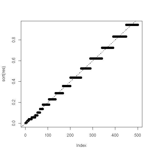
If the proposed median is wront, the p-values will be much lower.
N <- 500
n <- 10
res <- rep(NA,N)
for (i in 1:N) {
  res[i] <- sign.test(rlnorm(n),mu=2)
}
plot(sort(res), ylim=c(0,1))
abline(0,1/N,lty=2)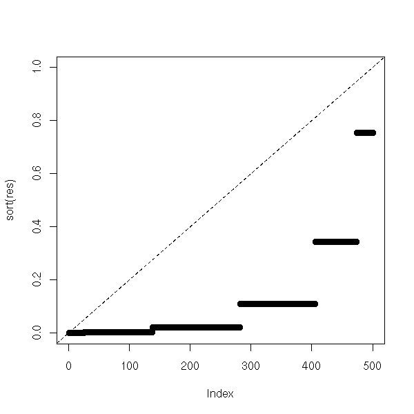
We can now complete our function to have confidence intervals.
sign.test <- function (x, mu=0, alpha=0.05) {
  n <- length(x)
  y <- sum(x<mu) # should warn about ties!
  p.value <- min(c( pbinom(y,n,.5), pbinom(y,n,.5,lower.tail=F) ))*2
  x <- sort(x)
  q1 <- qbinom(alpha/2,n,.5,lower.tail=T)
  q2 <- qbinom(alpha/2,n,.5,lower.tail=F)
  ci <- c(x[q1], x[q2])
  new.alpha = pbinom(q1,n,.5) + (1-pbinom(q2,n,.5))
  list(p.value=p.value, ci=ci, alpha=new.alpha)
}
We can check that the confidence intervals actually have the advertised risk (as the binomial distribution is a discrete distribution, this risk will not be exactly 0.05, that is why the function returns the theoretical value).
test.sign.test <- function (n=100, N=500) {
  N <- 500
  res <- matrix(NA, nr=N, nc=3)
  n <- 100
  for (i in 1:N) {
    r <- sign.test(rlnorm(n))
    ci <- r$ci
    res[i,] <- c( ci[1]<1 & 1<ci[2], n, r$alpha )
  }
  c(
     1-sum(res[,1], na.rm=T)/sum(!is.na(res[,1])),
     res[1,3]
   )
}

N <- 10
res <- matrix(NA, nc=3, nr=N, dimnames=list(NULL,
  c("Empirical Value", "Theoretical Value", "n")) )
for (i in 1:N) {
  n <- sample(1:200, 1)
  res[i,] <- round(c( test.sign.test(n), n ), digits=2)
}
res
This yields:
> res
       Empirical Value Theoretical Value   n
 [1,]             0.06              0.05  96
 [2,]             0.04              0.05 138
 [3,]             0.05              0.05   6
 [4,]             0.06              0.05 135
 [5,]             0.03              0.05 138
 [6,]             0.04              0.05  83
 [7,]             0.03              0.05 150
 [8,]             0.05              0.05  91
 [9,]             0.05              0.05 144
[10,]             0.04              0.05 177
TODO: read and correct (if needed) this part.
It is a non-parametric test: we do not know (or assume) anything on the distribution of the variables, in particular, we think it is not gaussian (to check ot, look at a quantile-quantile plot or perform a Shapiro--Wilk test) -- otherwise, we would use Student's T test, that is more powerful.
However, there IS an assumption: the variable is symetric (if it is not, consider the sign test). For this reason, we can speak of mean or of median -- for the whole distribution it is the same (but for a sample, that may be asymetric, it is different).
TODO: the following descrition is not that of the Wilcoxon
test I know, that assumes the variable is symetric, that
considers the variables Xij=(Xi+Xj)/2 and counts the
number of those variables that are above the proposed
mean.
The recipe is as follows. Take two samples, concatenate them, sort them. Then, look of the two samples are "well-shuffled" or if the elements from one sample are rather at the begining while those of the others are rather at the end.
The null hypothesis is H0: "P(X1_i > X2_i) = 0.5".
We first sort each sample (separately) and compute
U1 = number of pairs (i,j) such that X1_i>X2_j
     + (1/2) * number of pairs (i,j) so that X1_i=X2_j
U2 = number of pairs (i,j) so that X1_j>X2_i
     + (1/2) * number of pairs (i,j) so that X1_i=X2_j
U = min(U1,U2)
Here is another method of computing this:
Contatenate the two samples, rank them
R1 = sum of the ranks on the first sample
R2 = sum of the ranks on the second sample
U2 = n1*n2 + n1(n1+1)/2 - R1
U1 = n1*n2 + n2(n2+1)/2 - R2
U = min(U1, U2)
Here is example from the man page (here, we imagine that prior data suggests that x>y, so we choose an asymetric alternative hypothesis).
help.search("wilcoxon")
?wilcox.test
> x <- c(1.83,  0.50,  1.62,  2.48, 1.68, 1.88, 1.55, 3.06, 1.30)
> y <- c(0.878, 0.647, 0.598, 2.05, 1.06, 1.29, 1.06, 3.14, 1.29)
> wilcox.test(x, y, paired = TRUE, alternative = "greater", conf.level=.95, conf.int=T)

      Wilcoxon signed rank test

data:  x and y
V = 40, p-value = 0.01953
alternative hypothesis: true mu is greater than 0
95 percent confidence interval:
 0.175   Inf
sample estimates:
(pseudo)median
        0.46
Let us check on an example that the test remains valid for non-gaussian distributions.
N <- 1000
n <- 4
v <- vector()
w <- vector()
for (i in 1:N) {
  x <- runif(n, min=-10, max=-9) + runif(n, min=9, max=10)
  v <- append(v, wilcox.test(x)$p.value)
  w <- append(w, t.test(x)$p.value)
}
sum(v>.05)/N
sum(w>.05)/N
We get 1 and 0.93: we make fewer mistakes with Wilcoxons's test, but its power is lower, i.e., we miss many opportunities of rejecting the null hypothesis:
# Probability of rejecting H0, when H0 is false (power)
N <- 1000
n <- 5
v <- vector()
w <- vector()
for (i in 1:N) {
  x <- runif(n, min=0, max=1)
  v <- append(v, wilcox.test(x)$p.value)
  w <- append(w, t.test(x)$p.value)
}
sum(v<.05)/N
sum(w<.05)/N
We get 0 (the power of the test is zero: it never rejects the null hypothesis -- if our sample is very small and we do not know anything about the distribution, we cannot say much) against 0.84.
Let us consider a more ungaussian distribution.
# Probability of rejecting H0, when H0 is false (power)
N <- 1000
n <- 5
v <- vector()
w <- vector()
for (i in 1:N) {
  x <- runif(n, min=-10, max=-9) + runif(n, min=9, max=10)
  v <- append(v, wilcox.test(x)$p.value)
  w <- append(w, t.test(x)$p.value)
}
sum(v<.05)/N
sum(w<.05)/N
We get 0 and 0.05. For n=10, we would get 0.05 in both cases.
Let us now check the confidence interval.
N <- 1000
n <- 3
v <- vector()
w <- vector()
for (i in 1:N) {
  x <- runif(n, min=-10, max=-9) + runif(n, min=9, max=10)
  r <- wilcox.test(x, conf.int=T)$conf.int
  v <- append(v, r[1]<0 & r[2]>0)
  r <- t.test(x)$conf.int
  w <- append(w, r[1]<0 & r[2]>0)
}
sum(v)/N
sum(w)/N
We get 0.75 and 0.93.
TODO:

I do not understand.
As the U test is non-parametric, to should give larger
confidence intervals and make fewer mistakes.

The confidence interval for the Wilcoxon is three times as
small as that of Student's T test.

???

However, these simulations show that Student's T test is robust.

TODO: read what I just wrote and check the power
The following example tests if the variable is symetric around its mean.
> x <- rnorm(100)^2
> x <- x - mean(x)
> wilcox.test(x)

      Wilcoxon signed rank test with continuity correction

data:  x
V = 1723, p-value = 0.005855
alternative hypothesis: true mu is not equal to 0
Idem for the median.
> x <- x - median(x)
> wilcox.test(x)

      Wilcoxon signed rank test with continuity correction

data:  x
V = 3360.5, p-value = 0.004092
alternative hypothesis: true mu is not equal to 0
If there are more that two samples, you can use the Kruskal--Wallis test.
?kruskal.test
We want to see if two (quantitative random variables) follow the same distribution.
> ks.test( rnorm(100), 1+rnorm(100) )

      Two-sample Kolmogorov-Smirnov test

data:  rnorm(100) and 1 + rnorm(100)
D = 0.43, p-value = 1.866e-08
alternative hypothesis: two.sided

> ks.test( rnorm(100), rnorm(100) )

      Two-sample Kolmogorov-Smirnov test

data:  rnorm(100) and rnorm(100)
D = 0.11, p-value = 0.5806
alternative hypothesis: two.sided

> ks.test( rnorm(100), 2*rnorm(100) )

      Two-sample Kolmogorov-Smirnov test

data:  rnorm(100) and 2 * rnorm(100)
D = 0.19, p-value = 0.0541
alternative hypothesis: two.sided
TODO: state the idea (If my memory is good, we consider the sample cumulative distribution function of both variables and compute the area between them).
This test check if a random variable is gaussian. That might seem to be a special case of the Kolmogorov--Smirnov test, but actually we compare a random variable with the family of gaussian distributions, without specifying the mean and variance, while the K-S test want a completely specified distribution.
> shapiro.test(rnorm(10))$p.value
[1] 0.09510165
> shapiro.test(rnorm(100))$p.value
[1] 0.8575329
> shapiro.test(rnorm(1000))$p.value
[1] 0.1853919
> shapiro.test(runif(10))$p.value
[1] 0.5911485
> shapiro.test(runif(100))$p.value
[1] 0.0002096377
> shapiro.test(runif(1000))$p.value
[1] 2.385633e-17
It is a good idea to look at the quantile-quantile plot to see what happens, because the data might be non-gaussian in a benign way (either, as here, because the data are less dispersed that gaussian data, either because the deviation from a gaussian is statistically significant but practically negligible -- quite common if the sample is very large).
There is a wealth of other tests, we shall not detail them and merely refer to the manual.
?kruskal.test
?ansari.test
?mood.test
?fligner.test
library(help=ctest)
help.search('test')
TODO: State the structure of this part -- and reorder it...
1. Generalities about estimators
2. Least Squares estimators. Example: NLS.
3. Maximum Likelihood Estimators (also: REML, Penalized Likelihood)
4. GMM Estimators
Quite often, the data we are studying (the "statistical series") is not the whole population but just a sample of it -- e.g., when you study birds on an island, you will not measure all of them, you will simply catch a few dozen specimens and work on them. You can easily compute the statistical parameters of this sample (mean, standard deviation, etc.), but they are only approximations of those parameters for the whole population: how can we measure the precision of those approximations?
Here are a few concrete examples of this situation.
An industrialist must choose a variety of maize. It will be used as (part of) an animal food and we want the variety that contains the most proteins: we want to know the average protein content of each variety -- not that of the sample at hand, but that of the variety as a whole. We might find that the sample of a variety has a larger protein content that the sample of another: but were to samples sufficiently large, was the difference sifficiently significant to extrapolate the results to the whole population?
An industrialist must choose a variaty of maize. It will be sold for human consumption and, to ease its conditioning and packaging, we want all the ears to have the same size; i.e., we want the standard deviation to be as small as possible. If we find that the standard deviation of the sample of a variety is smaller than that of another variety, can we extrapolate the results to the varieties as a whole? Were the samples sufficiently large? Was the difference of standard deviations significant?
In simple terms: we draw, at random, subjects from a population and we measure, on the resulting sample, the statistical variables of interest (size, protein content, etc.).
In algorithmic terms:
Repeat a large number of times:
  Take a sample from the population
  Estimate, on this sample, the quantity of interest
  (this quantity is called a "statistic")
Compare those estimations (you can spot them as a histogram)
with the value on the whole population.
In more mathematical terms: Let X1,X2,...,Xn be independant identically distributed random variables (iidrv). With the value those variables take on a single point of the universe, we try to get some information about the distribution of those variables. For instance, we expect (X1+...+Xn)/n to be an estimation of the mean of this distribution: is it really the case? In what sense is it an "estimation"? What is the law of this sample mean? How to measure the quality of this estimation?
Let us consider a statistical experiment, i.e., iidrv X1,X2,...,Xn; we assume we know the family this distribution belongs to but not its parameters (for instance, we know it is a gaussian distribution, but we do not know the mean, or the variance -- or even both). An estimator is a function of X1,X2,...,Xn that gives an estimation of this parameter. (If we see the random variables X1,X2,...,Xn as maps from the universe Omega to the real line R, an estimator is the random variable obtained by composing (X1,...,Xn) with a map R^n ---> R.) For instance, (X1+...+Xn)/n is an estimator of the mean.
(Remark: we said that it was an estimator of the mean, but nowhere in the definition did the mean appear. Indeed, it is also an estimator of the variance, of the standard deviation or of any quantity we could think of -- but we will see shortly that is is a "good" estimator of the mean and a bad estimator of all these other quantities.)
Quite often, estimators comes in families; for instance, the formula (X1+...+Xn)/n is a family of estimators of the mean: we have one for each n.
It is an estimator whose expectation is indeed the value of the parameter. For instance, the sample mean (X1+...+Xn)/n is indeed an unbiased estimator of the mean. On the contrary, the variance of the sample is a biased estimator of the population variance (but you can easily transform it into an unbaised estimator: just replace "n" in the denominator by "n-1").
We can check this with a small simulation, as follows.
Let us draw 5 numbers at random, following a gaussian distribution of mean 0 and variance 1.
If we repeat this experiment 10000 times, we get (an estimation of) the expectation the empirical mean: it is roughly equal to the population mean (here, 0).
x <- vector()
for(i in 1:10000){
  x <- append(x, mean(rnorm(5)))
}
mean(x)

[1] 9.98948e-05
If we proceed likewise with the variance, we see that its expectation is significantly different from the population variance (we get 0.8 instead of 1): we say that the "population variance" is a biased estimator of the population variance.
TODO: the last paragraph was a bit ambiguous...
n <- 5
x <- vector()
for(i in 1:10000){
  t <- rnorm(n)
  t <- t - mean(t)
  t <- t*t
  x <- append(x, sum(t)/n)
}
mean(x)

[1] 0.806307
To get an unbiased estimator of the variance, it suffices to replace the "n" in the definition of the variance by "n-1". These two notions of variance are called "population variance" and "sample variance".
                       1
Population variance = --- * Sum( X_i - mean(X_j) )
                       n     i

                        1
    Sample variance = ----- * Sum( X_i - mean(X_j) )
                       n-1     i
Let us check, with another simulation, that this is indeed unbiased.
n <- 5
y <- vector()
for(i in 1:10000){
  t <- rnorm(n)
  t <- t - mean(t)
  t <- t*t
  y <- append(y, sum(t)/(n-1))
}
mean(y)

[1] 1.000129
But this is not the only unbiased estimator of the variance: if we use the first formula with the actual mean (that of the population, not that of the sample), the estimator is indeed unbiased (but this is unrealistic: there is no reason why we should know the population mean).
n <- 5
z <- vector()
for(i in 1:10000){
  t <- rnorm(n)
  t <- t - 0
  t <- t*t
  z <- append(z, sum(t)/n)
}
mean(x)

[1] 1.001210
We can graphically compare those three estimators of the variance.
n <- 5
x <- y <- z <- vector()
for(i in 1:10000){
  t <- rnorm(n)
  z <- append(z, sum(t*t)/n)
  t <- t - mean(t)
  t <- t*t
  x <- append(x, sum(t)/n)
  y <- append(y, sum(t)/(n-1))
}
boxplot(x,y,z)
plot(density(x))
points(density(y), type="l", col="red")
points(density(z), type="l", col="blue")

op <- par( mfrow = c(3,1) )
hist(x, xlim=c(0,5), breaks=20)
hist(y, xlim=c(0,5), breaks=20)
hist(z, xlim=c(0,5), breaks=20)
par(op)
Their square root (three estimators of the standard deviation) is more symetric.
x <- sqrt(x)
y <- sqrt(x)
z <- sqrt(z)
boxplot(x,y,z)
plot(density(x))
points(density(y), type="l", col="red")
points(density(z), type="l", col="blue")
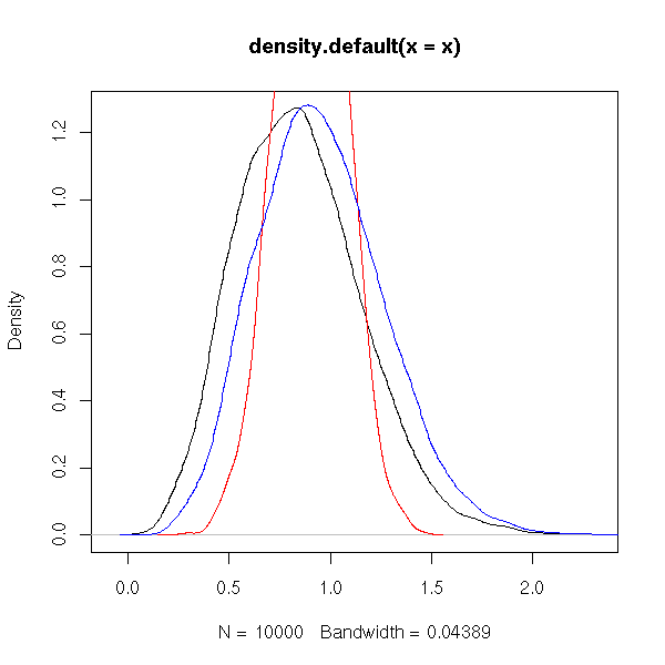
op <- par( mfrow = c(3,1) )
hist(x, xlim=c(0,5), breaks=20)
hist(y, xlim=c(0,5), breaks=20)
hist(z, xlim=c(0,5), breaks=20)
par(op)
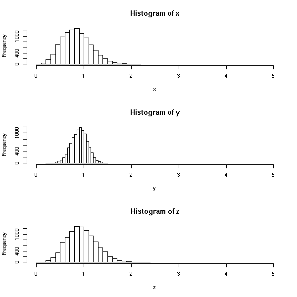
Question: are these estimators of the standard deviation biased? Check your answer with a few simulations. Do you understand why? (Hint: they are all biased. The expectation is an integral and we know that, in general, the integral of a square root is not the square roor of the integral.)
TODO: check this hint.
There are many other notions, besides bias, that measure the quality of an estimator or of a sequence of estimators. For instance, an estimator is "consistent" if, when the sample size grows, ot converges (in probability) to the desired value. Thus, the weeak law of large numbers states that the sample mean is a consistent estimator of the population mean.
But where do we find the estimators in the first place? For simple quantities, such as the mean or the variance, we have a formula for the whole population and we hope it will work for a sample. For the mean, it works; for the variance, it yields a biased estimator, but we can tweak it into an unbiased one.
But if we want to find a parameter of a more complicated law, for which we have no "population formula" (imagine, for instance, that you want to find the parameter(s) of an exponential, Poisson, Gamma, Beta, Weibull, Binomial, etc. distribution), how do we proceed?
The Maximum Likelihood is a recipe to find such a candidate estimator. We do not know of it will have "good" properties, in particular, it will pften be biased, it it will be a good start. The idea is to find the value of the parameter for which the probability of observing the results actually observed in the sample is maximum -- this quantity is called the "likelihood": we maximize it.
For instance, let us use this method to find an estimator if the mean of a gaussian random variable of variance 1 with a 5-element sample (actually, in this case, we get the "sample mean" -- the method is useful in more complex situations).
# The population mean
m <- runif(1, min=-1, max=1)
# The n-element sample
n <- 5
v <- rnorm(n, mean=m)
# Likelihood
N <- 1000
l <- seq(-2,2, length=N)
y <- vector()
for (i in l) {
  y <- append(y, prod(dnorm(v,mean=i)))
}
plot(y~l, type='l')
# Population mean
points(m, prod(dnorm(v,mean=m)), lwd=3)
# Sample mean
points(mean(v), prod(dnorm(v,mean=mean(v))), col='red', lwd=3)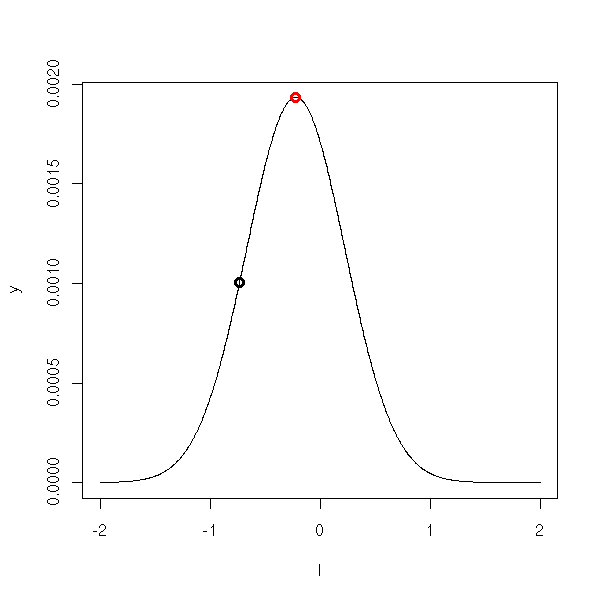
The "optimize" function finds such a maximum, in dimension 1.
> optimize(dnorm, c(-1,2), maximum=T)
$maximum
[1] 1.307243e-05
$objective
[1] 0.3989423
In higher dimensions, you can use the "optim" function (it looks for a minimum)
f <- function (arg) {
  x <- arg[1]
  y <- arg[2]
  (x-1)^2 + (y-3.14)^2
}
optim(c(0,0), f)
of the "nlm" function
TODO
We get:
$par
[1] 0.9990887 3.1408265

$value
[1] 1.513471e-06

$counts
function gradient
      59       NA

$convergence
[1] 0

$message
NULL
We can ask for a specific optimization method, for instance, simulated annealing -- actually, in this example, we get an imprecise result.
optim(c(0,0), f, method="SANN")
Let us consider the eruption lengths of the Faithful geyser and let us try to approximate them as a mixture of Gaussian variables.
f <- function (x, p, m1, s1, m2, s2) {
  p*dnorm(x,mean=m1,sd=s1) + (1-p)*dnorm(x,mean=m2,sd=s2)
}
data(faithful)
fn <- function(arg) {
  prod(f(faithful$eruptions, arg[1], arg[2], arg[3], arg[4], arg[5]))
}
start <- c(.5,
           min(faithful$eruptions), var(faithful$eruptions),
           max(faithful$eruptions), var(faithful$eruptions),
          )
p <- optim(start, function(a){-fn(a)/fn(start)}, control=list(trace=1))$par
hist(faithful$eruptions, breaks=20, probability=T, col='light blue')
lines(density(faithful$eruptions,bw=.15), col='blue', lwd=3)
curve(f(x, p[1], p[2], p[3], p[4], p[5]), add=T, col='red', lwd=3)
#curve(dnorm(x, mean=p[2], sd=p[3]), add=T, col='red', lwd=3, lty=2)
#curve(dnorm(x, mean=p[4], sd=p[5]), add=T, col='red', lwd=3, lty=2)
legend(par('usr')[2], par('usr')[4], xjust=1,
       c('sample density', 'theoretical density'),
       lwd=3, lty=1,
       col=c('blue', 'red'))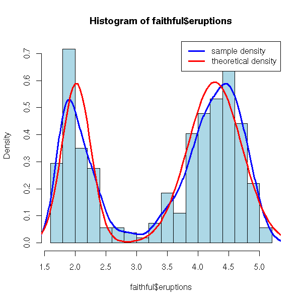
We have just seen, in the previous examples, that the likelihood was often defined as a product, with as many factors as observations. As such large products are numerically unwieldy, we often prefer to take their logarithm.
TODO: the "fitdistr", in the MASS package, computes univariate maximum likelihood estimators.
TODO: The "mle" function in the "stats4" package is a wrapper around "optim" and provides functions to compute the information matrix, the covariance matrix, confidence intervals, etc.
The log likelihood is (not the logarithm of the likelihood but)
-2 log (vraissemblance).
It is the quantity we try to minimize in the Maximum likelihood method.
You might wonder where the "-2" coefficient comes from: for gaussian variables, it yields the logarithm of the sum of squares.
TODO: check the above.
If L is the log-likelihood and p the parameter to estimate, then the "score" is defined as
     d log L
U = ---------
       d p
and the Fisher information as
        d^2 L
I(p) = -------
        d p^2
The Fisher information measures the sharpness of the peak at the maximum of L.
TODO: I have NOT said anything about "H0" and "H1"...
We remark that
              L if H0 is true
LR = - 2 log ---------------------------------------
              L with the MLE parameters

              L(b0)
   = - 2 log -------  (if b is the parameter to estimate)
              L(b)
where L is the likelihood, approximately follows a Chi^2 distribution with m degrees of freedom, where m is the number of parameters to estimate.
TODO: explain why, in the gaussian case, it IS a Chi^2
distribution
TODO: explain how we estimate the variance of the
estimator.

TODO: an example (take one gaussian distribution and model
it as a mixture of distributions; take a mixture of two
gaussian distributions and model it as a mixture of two
gaussians; in both cases, test if the means of the two
gaussian distributions are the same).
The "Wald test" and the "score test" are approximations of the Likelihood Ratio (LR) test. More precisely, if we note b the parameter to estimate, the "score" (it is a vector) is
U(b) = Nabla log V(b)

       (  d log V(b)  )
     = ( ------------ )
       (     d bi     ) i
and the "information" (it is a matrix) is
       (       d^2              )
I(b) = ( - ----------- log V(b) )
       (    d bi d bj           ) i,j
The "Wald statistic" is an order 2 Taylor expansion of the Likelihood Ratio (LR)
W = (b-b0)' * I(b) * (b-b0)
and the "Score statistic" (it does not depend on b: it is very imprecise, but very fast to compute)
S = U(b0)' * I(b0)^-1 * U(b0).
We can see the likelihood as the probability density function of the parameter, conditionnal to the sample.
TODO: is it true?
TODO: plot
The idea of the Maximum Likelihood Method is to take the mode of this function. But there are a few problems.
First, we completely forget the distribution of this estimator: we often look at its variance, but if it is not normal, this is far from sufficient. (We can use this density to measure the quality of the estimator or to do simulations (parametric bootstrap)).
Besides, the mode is not always a good choice. Why not take the mean (this is called bagging -- more about this later) or the median? What do we do if the mode is not unique? Or, more realistically, if the likelihood has several local maxima? Or a high narrow peak (so narrow that its probability is low) and a wider smaller peak (so that its probability is high)?
op <- par(mfrow=c(2,2))
curve(dnorm(x-5)+dnorm(x+5), xlim=c(-10,10))
curve(dnorm(x-5)+.4*dnorm(x+5), xlim=c(-10,10))
curve(dnorm(5*(x-5)) + .5*dnorm(x+5), xlim=c(-10,10))
par(op)
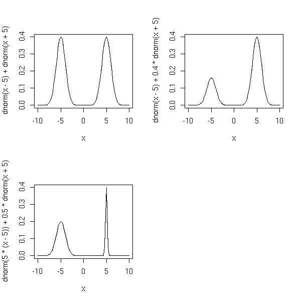
However, I have not managed to devise a situation in which we really observe such a phenomenon (if you have such an example, tell me). Actually, such a situation might be a sign that the model is wrong.
Ah, I finally got such an example. I simply took an estimator you cannot extrapolate from a sample to a population: the maximum. (The statistics for which we might want to find an estimator might have, or not, pleasant properties: the maximum is one of the worst statistics you can imagine.)
get.sample <- function (n=10, p=1/100) {
  ifelse( runif(n)>p, runif(n), 2 )
}
N <- 1000
d <- rep(NA,N)
for (i in 1:N) {
  d[i] <- max(get.sample())
}
hist(d, probability=T, ylim=c(0, max(density(d)$y)), col='light blue')
lines(density(d), type='l', col='red', lwd=3)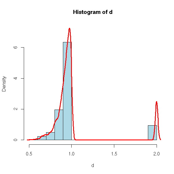
get.sample <- function (n=100, p=1/100) {
  ifelse( runif(n)>p, runif(n), 2 )
}
N <- 1000
d <- rep(NA,N)
for (i in 1:N) {
  d[i] <- max(get.sample())
}
#hist(d, breaks=seq(0,3,by=.02),
#     probability=T, ylim=c(0, max(density(d)$y)), col='light blue')
#lines(density(d), type='l', col='red', lwd=3)
plot(density(d), type='l', col='red', lwd=3)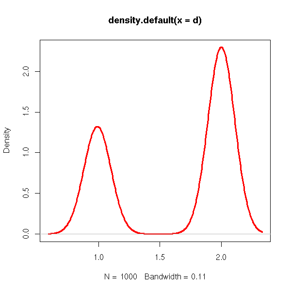
get.sample <- function (n=100, p=1/100) {
  ifelse( runif(n)>p, runif(n), 2+2*runif(n) )
}
N <- 1000
d <- rep(NA,N)
for (i in 1:N) {
  d[i] <- max(get.sample())
}
#hist(d, breaks=seq(0,4,by=.05),
#     probability=T, ylim=c(0, max(density(d)$y)), col='light blue')
#lines(density(d), type='l', col='red', lwd=3)
plot(density(d), type='l', col='red', lwd=3)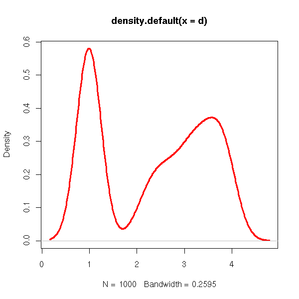
However, some methods replace the estimators (a single value) by probability distributions: on the computational side, all the methods relying on the bootstrap (e.g., the bagging), on the theoretical side, these are called "bayesian methods".
We have just seen that it could be interesting to have, not an estimator (a single number, possibly with its variance) but a whole probability distribution. Bayesian methods push this remark a little further.
We assume that the parameters of the model were chose at random according to a given distribution -- the prior distribution. Bayesian methods try fo find the posterior distribution, i.e., the distribution of those parameters given the actually observed sample.
TODO: write this up.
Z: date
t: parameters
The model gives us P(Z|t)
We assume we know P(t) (the prior distribution).
We then compute P(t|Z) (posterior distribution) from P(Z|t) and
P(t), with the Bayes formula -- hence the name.

TODO: recall this formula.

TODO:
MCMC (Markov Chain Monte Carlo) to sample from the posterior distribution
parametric bootstrap = computational implementation of the maximum likelihood method
MLE = mode
bagged estimator = mean

TODO: EM algorithm (to find MLE in a 2-component misture model)
1. find first estimates (m1, m2: random; s1, s2: sd(whole sample))
2. Compute the responsabilities
   gamma(i) = probability that observation i comes from the second component
   1-gamma(i)=probability that observation i comes from the first component
3. new estimators = weighted means and variances
   (use gamma(i), resp 1-gamma(i), as weights)
4. Iterate

TODO: you can generalize this algorith to other models.

TODO: this is a special case of REML

TODO: put those more complicated examples in the "bootstrap" chapter/section?

TODO: remark that bayesian methods can be applied iteratively.
  Initial data --> prior
  New data --> posterior
  Update prior
  New data --> posterior
  Update prior
  ...

TODO: The theory behind the Kalman Filter (State Space
Models) is bayesian.
Bayesian statistics are very similar to quantum mechanics: in quantum mechanics, reality is a superposition of many possible realizations, each with its probability; similarly, the result of a bayesian analysis is a whole probability distribution, giving all the possible answers, each with its probability.
TODO
This is very similar to neural networks, but we can
interpret the resulting model and add (prior) information
to it.
TODO
(Notes taken while reading Matlab's documentation)
The idea behind Fuzzy Inference Systems is to replace boolean values by continuously varying values -- think "probabilities".
curve(ifelse(x < .3, 0, ifelse(x > .7, 0, 1)),
      lwd = 3, col = "blue",
      xlim = c(0,1),
      main = "A classical membership function",
      xlab="", ylab="")
abline(h = 0, lty = 3)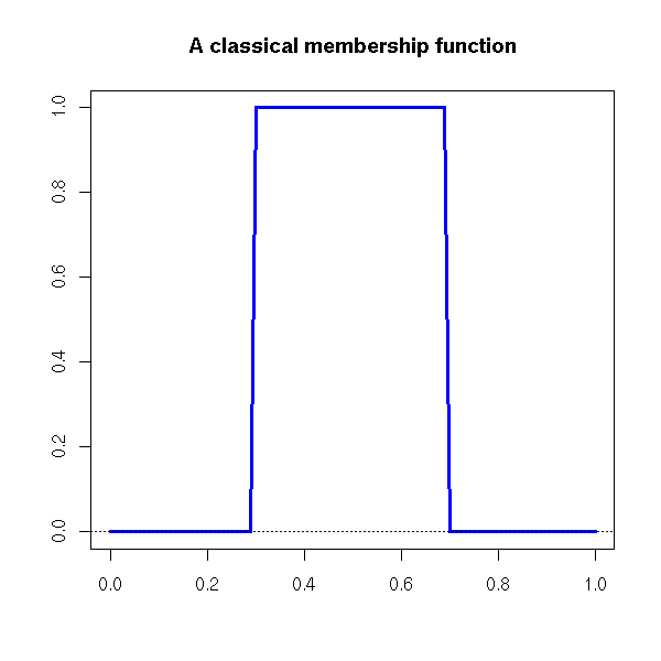
curve( dnorm( x - .5, sd = .1 ) / dnorm(0, sd=.1),
       lwd = 3, col = "blue",
       xlim = c(0, 1),
       main = "A fuzzy membership function",
       xlab="", ylab="" )
abline(h=0, lty=3)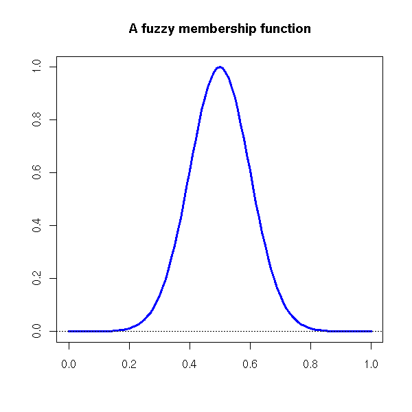
Boolean operators and deduction rules can then be fuzzified: AND becomes MIN, OR becomes MAX, NOT(x) becomes 1-x THEN becomes MIN.
Note that there might be incoherences in the rules -- it is not a problem.
You can tune the fuzzy inference system by changing the
membership functions (or even the boolean operators).
As with bayesian methods, the result is a probability
distribution, not a single number.
So far, it looks like bayesian networks, with a very
simple, fixed network structure, and no learning
capabilities.

(2) Adaptive Neuro-Fuzzy Inference Systems (ANFIS)
Actually, you do not have to provide the set of rules: you
can simply take you data, cluster it, and ask the computer
to write a rule for each cluster.
This looks very similar to nearest-neighbour methods --
and, if you impose some parsimony, it can be seen as a
machine-learning analogue of Generalized Additive Models
(GAM, "mgcv" package in R).

(3) Fuzzy C-means clustering
This is a generalization of the k-means clustering
algorithm where cluster membership is fuzzy -- i.e., is a
probability. (In R, ir is implemented in the "fanny" or
"cmeans" functions.)
Let us consider an extimator U of a parameter u of a distribution F(u). The problem, is that we do not know F exactly (more realistically: we do know F, but the population does not exactly follow this distribution, it is merely an estimation of the distribution of the data). To assess the robustness of the estimator, we can check how it changes when we modify F at a single point. More precisely, we compute
                U( (1-h) F + h 1x ) - U(F)
w(x) =   lim   ----------------------------
       h -> 0              h
Where 1x is the Dirac measure at x.
TODO: example with the mean
TODO: example with the variance
TODO: example with the correlation (in dimension 2)
?persp
TODO: empirical estimation of the influence function with bootstrap.
library(boot)
?empinf
TODO: TO SORT?
This is another recipe to get an estimator. If there is a single parameter, we choose it so that the first moment (i.e., the mean) of the variable coincides with the sample mean. If there are k parameters, we choose them so that the first k moments coincide with the sample moments (I recall that the moments of a real random variable X are the expectations of X^k). As with the Maximum Likelihood Method, we do not know anything about the quality of the resulting estimator -- it is often biased.
Let us use this method to study the Faithful geyser eruptions durations. Let X0 be a Bernoulli random variable (i.e., a rnadom variable with two values, 0 and 1, or "heads" and "tails"), with parameter p, and X1, X2, gaussian random variables of mean m1, m2 and standard deviations s1, s2. We try to put our data Y under the forn
Y = X0 X1 + (1-X0) X2.
Noting that X0^2=X0, (1-X0)^2=1-X0 et X0*(1-X0), one can show that
Y^2 = X0 X1^2 + (1-X0) X2^2
Y^3 = X0 X1^3 + (1-X0) X2^3
Y^4 = X0 X1^4 + (1-X0) X2^4.
As X0, X1, X2 are independant,
E(Y) = X(X0) E(X1) + E(1-X0) E(X2)
E(Y^2) = X(X0) E(X1^2) + E(1-X0) E(X2^2)
E(Y^3) = X(X0) E(X1^3) + E(1-X0) E(X2^3)
E(Y^4) = X(X0) E(X1^4) + E(1-X0) E(X2^4)
But as
E(X0)=p

E(X1) = m
E(X1^2) = m^2 + s^2
E(X1^3) = 3 m s^2 + m^3
E(X1^4) = 10 s^4 + 6 s^2 m^2 + m^4
E(X1^5) = 50 s^4 m + 5 s^2 m^3 + m^5
(and similarly for X2), we get
E(Y)   = p m1 + (1-p) m2
E(Y^2) = p (m1^2 + s1^2) + (1-p) (m2^2 + s2^2)
E(Y^3) = p (3 m1 s1^2 + m1^3) + (1-p) (3 m2 s2^2 + m2^3)
E(Y^4) = p (10 s1^4 + 6 s1^2 m1^2 + m1^4) + (1-p) (10 s2^4 + 6 s2^2 m2^2 + m2^4)
E(Y^4) = p (50 s1^4 m1 + 5 s1^2 m1^3 + m1^5) + (1-p) (50 s2^4 m2 + 5 s2^2 m2^3 + m2^5)
We can then ask R to find (numerically) the values of those five parameters).
(Exercise left to the reader -- I am not absolutely sure of my results.)
TODO
There is a function to find the minimum of a function of
several variables (optimize, optim, nlm, nls), there are
functions to find the zeros of a function of a single
variable (uniroot, polyroot), but what about the zeros of
a function of several variables, i.e., how do we
numerically solve a non-linear system???

(One can do that with the Newton algorithm, as in
dimension 1 -- the only difference being that the
derivative is a matrix.)
Since the higher moments have a high variance, are very sensitive to outliers -- or even, in some cases, are not defined for the distribution at hand --, one can replace the moments by the L-moments or the trimmed L-moments (TL-moments).
Least squares and maximum likelihood provide recipes to build new estimators. The Generalized Method of Moments is another recipe, that actually generalizes both Least Squares and Maximum Likelihood.
Consider a (real-valued) random variable X, known to be gaussian, with unknown mean mu and standard deviation sigma. We want to find those parameters, mu and sigma, from a sample x1,x2,...,xn, drawn from the distribution of X. Remarking that
E[ X ] = mu
E[ X^2 ] = mu^2 + sigma^2
we can simply try to solve
 1
--- Sum( x_i ) = mu
 n

 1
--- Sum( x_i^2 ) = mu^2 + sigma^2
 n
There is no reason it will be a "good" estimator, but it will be an estimator -- then, it is up to us to study how good it is and to improve it if needed.
This idea is more general: if the distribution of the random variable X has a known form, with unknown parameters theta_1, theta_2, ..., theta_n, we can compute the first moments of X as a function of those parameters
E[ X   ] = m_1( theta_1, ..., theta_n )
E[ X^2 ] = m_2( theta_1, ..., theta_n )
E[ X^3 ] = m_3( theta_1, ..., theta_n )
...
Then, given the value of X on a sample, we can equate the mean of X, X^2, etc. to their theoretical values and solve the resolving equations. This is called the Method of Moments Estimator (MME).
But this can be generalized further: instead of taking the moments E[X], E[X^2], E[X^3], etc., we can consider the expectation of simpler quantities, that have a more direct interpretationm or that can be more easily computed. Those quantites are called generalized moments.
The recipe for our more GMM estimator is: find easy-to-compute and easy-to-interpret quantities (e.g., X, X^2, X^3, etc.); compute their expectation in the population, as functions of the unknown parameters; compute their average in the sample; equate expectations and averages and solve: the law of large numbers tells you that the averages converge to the expectations. Furthermore, the law of large numbers (often) tells you that the resulting estimators are asymptotically gaussian.
For instance, if you have two random variables X and Y, linked by the relation Y = a + b X + epsilon, where epsilon is a random variable with zero mean and a and b are unknown parameters, then you can consider the generalized moments
E[ Y - ( a + b X ) ]     = 0
E[ (Y - ( a + b X )) X ] = 0
The corresponding GMM estimator is the least squares estimator: the equations state that the derivatives the of sum of squares appreaing the the definition of the least squares estimator with respect to X and Y are zero.
The classical moments can be written as
E[ X   - m1(theta) ] = 0
E[ X^2 - m2(theta) ] = 0
E[ X^3 - m3(theta) ] = 0;
...
we shall write the generalized moments as
E[ h1(X, theta) ] = 0
E[ h2(X, theta) ] = 0
E[ h3(X, theta) ] = 0
...
Quite often, you have more generalized moments than parameters: in this case, you cannot hope that the moments will all be zero, and you will try to minimize a "weighted sum" of squares of generalized moments. More precisely, if h = (h1,...,hn) is the vector of generalized moments, you will minimize
h' W h
where W is a weight matrix. If you are completely clueless about the properties of your moments, you can set W to the identity matrix, but otherwise, the (limit, when the sample size becomes large, of the) inverse of the variance-covariance matrix of the residuals is a good choice
W = Var[ (1/N) Sum( h(x_i, theta) ) ] ^ -1
The actual algorithm is usually:
W <- I
Until convergence:
  Find theta that minimizes [(1/N)Sum(h(x_i))]' W [(1/N)Sum(h(x_i))]
  Set W = Var[residuals]^-1
TODO: Orthogonality conditions, Instrumental Variables (IV)
When you select you model, say Y = f(X, theta) + epsilon,
you want its residuals to be uncorrelated with all the
predictive variables, say
  epsilon = y - f(x, theta)    uncorrelated with x (variables
                               included in the model)
  epsilon = y - f(x, theta)    uncorrelated with z (variables
                               not included in the model)

The first condition will be satisfied, but the second need
not: we have to impose it. This can be written as
  E[ (y - f(x, theta)) \tens z ] = 0
where \tens is the tensor product (also called "Kroneker
product").

TODO: recall what it is.

The variables in z (the columns of z) are called
Instrument Variables (IV).
Tests, in the context of the Generalized Method of Moments, can look as follows:
H0: E[ h ]  = 0, i.e., the model is right
H1: E[ h ] != 0, i.e., the model is wrong
You can use the following statistic:
J = N [(1/N)Sum(h(x_i))]' W [(1/N)Sum(h(x_i))]
where N is the sample size.
You should remark that, with the GMM, we never really specify the model: we just specify its moments. Thus, in this context, we cannot distinguish between models with the same moments.
GMM are used in econometrics, because one can choose moments with an economic interpretation -- furthermore, as there is no real model behind the moments, once the moments are meaningful, the "model" makes sense.
TODO: give more details
The Cramer-Rao inequality states that one cannot find arbitrarily good extimators: more precisely, it gives a lower bound on the variance of an unbiased estimator.
The first step to find the "best" estimator possible is to replace the data X1,X2,...,Xn by one (or several) numbers that contain as much information: this number is called a "sufficient statistic". More precisely, if
P( (X1,X2,...,Xn) \in U | t(X1,...,Xn) = c )
only depends on U and C but not on the parameter we want to estimate, then t is a sufficient statistic. There is a simple criterion (the Neyman factorization theorem) to recognize a sufficient statistic. More precisely, we try to find a "minimal" sufficient statistic, i.e., one whose "level lines" be as large as possible.
Unbiased estimators whose variance is the lower bound in the Cramer-Rao inequality.
TODO
The information of a realization of a random variable is its degree of surprise. For instance, if we flip a coin (i.e., if we consider a Bernoulli variable with probability 1/2) and get heads, there is no real surprise: the information is rather low. This notion becomes more interesting for more asymetric random variables. Let us consider the occurrence of an earthquake, given that earthquakes are rare. Knowing that no earthquake occurred is not informative at all: the information is low (even lower than in the coin flip experiment). On the contrary, if an earthquake did occur, this is surprising, and the information is high.
For a Bernoulli variable
P(X=1) = p
the information of the event X=1 is
TODO: formulas
TODO
The Kolmogorov-Chaitin entropy of a sequence of characters is the minimal length of a program that produces this sequence.
It cannot really be computed but, if your sequence is sufficiently long, you can estimate its entropy by compressing the sequence (with programs such as gzip or bzip2) and looking at the length of the resulting file.
http://arxiv.org/abs/cond-mat/0108530 Language trees and zipping
http://arxiv.org/abs/cond-mat/0202383 Extended comments on "Language trees and zipping"
http://arXiv.org/abs/cond-mat/0203275
TODO
TODO: write this part...
Likelihood-Ratio test
LR = -2 ln ( L at H0 / L at MLE )
LR ~ Chi2
df = number of parameters (eg, 1).

Other tests for MLE: Wald test, Score test.

To compare two models fitted with MLE, compare AIC = LRChi^2 - 2 p
where p is the number of parameters.  This is an approximative
criterion. There are other questionable such criteria, eg, BIC
(Bayesian Information Criterion).
r <- lm(...)
AIC(r)
library(nlme)
BIC(r)
r <- gls(...)
summary(r)

The AIC says that adding a useless parameter generally increases the
log likelihood by about 1 unit.
So if adding a parameter increases the log like- lihood by more than 1,
it is not useless.

This work is licensed under a Creative Commons Attribution-NonCommercial-ShareAlike 2.5 License.
Vincent Zoonekynd
<zoonek@math.jussieu.fr>
latest modification on Sat Jan 6 10:28:20 GMT 2007