
The zoo of discrete probability distributions
The zoo of continuous probability distributions
Fitting a distribution
Extreme value theory
Miscellaneous
In this chapter, we present the most important probability distributions (Gaussian, Exponential, Uniform, Bernoulli, Binomial, Poisson); we explain how to "fit" a distribution, i.e., how to find the distribution that most closely matches a given data set, i.e., how to find the most probable parameters; finally, we focus on the distributions of extreme values.
The most important discrete probability distributions are the Bernoulli, Binomial and Poisson distributions.
Tossing a coin is equivalent to examining a random variable following a Bernoulli distribution of parameter 0.5. If the coin has been tampered with and "heads" appears with probability p, it is a Bernoulli distribution of parameter p.
P( X=1 ) = p
P( X=0 ) = 1-p
In case of equiprobability, you can simulate such an experiment with the "sample" command, that performs such draws, with or without replacement, from a given set.
n <- 100
x <- sample(c(-1,1), n, replace=T)
plot(x, type='h', main="Bernoulli variables")

n <- 1000
x <- sample(c(-1,1), n, replace=T)
plot(cumsum(x), type='l',
     main="Cumulated sums of Bernoulli variables")
If the probabilities of both events are differents, we can still use the "sample" command, with one more argument.
n <- 100
x <- sample(c(-1,1), n, replace=T, prob=c(.2,.8))
plot(x, type='h',
     main="Bernoulli variables, different probabilities")
n <- 200
x <- sample(c(-1,1), n, replace=T, prob=c(.2,.8))
plot(cumsum(x), type='l',
     main="Cummulative sums of Bernoulli variables")
But you can also do than by hand, with the "runif" command.
n <- 200
x <- runif(n)
x <- x>.3
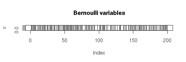
plot(x, type='h', main="Bernoulli variables")
This is a generalization of the Bernoulli distribution: we draw a number at random from 1, 2, ..., n.
We can simulate this distribution with the "sample" command.
> sample(1:10, 20, replace=T)
[1]  1  5  6  4  7  5  3  6  2  9 10 10  8  3 10  7  4  1  1  3
We toss a coin n times and we count the number of "heads".
In more formal terms: a Binomial variable of parameters (n,p) is a sum of n Bernoulli variables of parameter p.
We can simulate it as follows.
N <- 10000
n <- 20
p <- .5
x <- rep(0,N)
for (i in 1:N) {
  x[i] <- sum(runif(n)<p)
}
hist(x,
     col='light blue',
     main="Simulating a binomial law")
We can also use the "rbinom" command.
N <- 1000
n <- 10
p <- .5
x <- rbinom(N,n,p)
hist(x,
     xlim = c(min(x), max(x)),
     probability = TRUE,
     nclass = max(x) - min(x) + 1,
     col = 'lightblue',
     main = 'Binomial distribution, n=10, p=.5')
lines(density(x, bw=1), col = 'red', lwd = 3)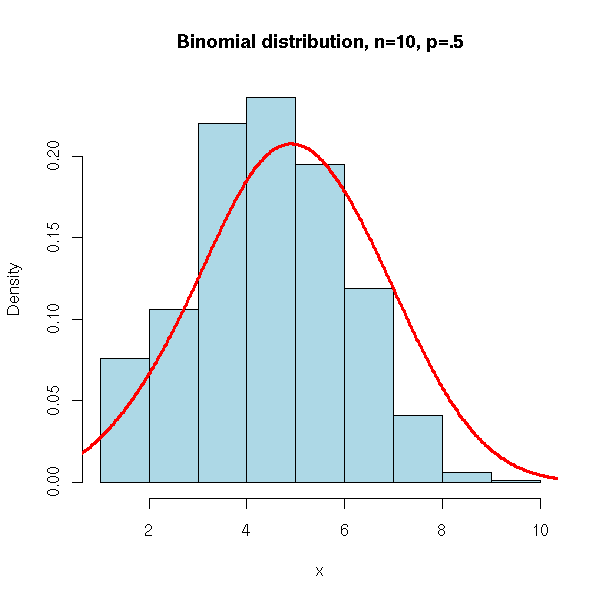
N <- 100000
n <- 100
p <- .5
x <- rbinom(N,n,p)
hist(x,
     xlim = c(min(x), max(x)),
     probability = TRUE,
     nclass = max(x) - min(x) + 1,
     col = 'lightblue',
     main = 'Binomial distribution, n=100, p=.5')
lines(density(x,bw=1), col = 'red', lwd = 3)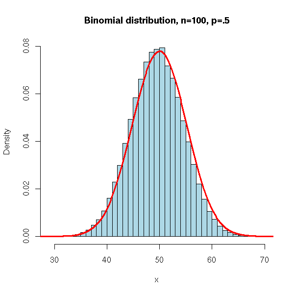
p <- .9
x <- rbinom(N,n,p)
hist(x,
     xlim = c(min(x), max(x)),
     probability = TRUE,
     nclass = max(x) - min(x) + 1,
     col = 'lightblue',
     main = 'Binomial distribution, n=100, p=.9')
lines(density(x,bw=1), col = 'red', lwd = 3)
It is also the distribution of the number of red balls sampled with replacement from an urn containing red and black balls: we can simulate it with the "sample" command.
N <- 10000
n <- 100
p <- .5
x <- NULL
for (i in 1:N) {
  x <- append(x, sum(sample( c(1,0),
                             n,
                             replace = TRUE,
                             prob = c(p, 1-p) )))
}
hist(x,
     xlim = c(min(x), max(x)),
     probability = TRUE,
     nclass = max(x) - min(x) + 1,
     col = 'lightblue',
     main = 'Binomial distribution, n=100, p=.5')
lines(density(x,bw=1), col = 'red', lwd = 3)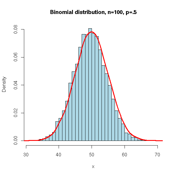
You will also meet this distribution in ecology, when you try to estimate the number of animals of a given species (say, fish in a lake). You catch the animal, you mark them (with a ring -- the word to google for is "ringing"), and afetr some time, a part of the population is ringed (we know how many, because we have counted the rings), the rest is not. When we catch new animals, we have a certain number of ringed animals and a certain number of non-ringed animals: we can use those numbers to estimate the population size.
This is the distribution of the number of red balls samples without replacement from an urn containing red and white balls.
Let us simulate it on an example: we sample without replacement 5 balls from an urn containing 15 white and 5 red balls and we count the number of white balls.
N <- 10000
n <- 5
urn <- c(rep(1,15),rep(0,5))
x <- NULL
for (i in 1:N) {
  x <- append(x, sum(sample( urn, n, replace=F )))
}
hist(x,
     xlim=c(min(x),max(x)), probability=T, nclass=max(x)-min(x)+1,
     col='lightblue',
     main='Hypergeometric distribution, n=20, p=.75; k=5')
lines(density(x,bw=1), col='red', lwd=3)
Alternatively, you can directly use the "rhyper" function (it is faster).
N <- 10000
n <- 5
x <- rhyper(N, 15, 5, 5)
hist(x,
     xlim=c(min(x),max(x)), probability=T, nclass=max(x)-min(x)+1,
     col='lightblue',
     main='Hypergeometric distribution, n=20, p=.75, k=5')
lines(density(x,bw=1), col='red', lwd=3)
N <- 10000
n <- 5
x <- rhyper(N, 300, 100, 100)
hist(x,
     xlim=c(min(x),max(x)), probability=T, nclass=max(x)-min(x)+1,
     col='lightblue',
     main='Hypergeometric distribution, n=400, p=.75, k=100')
lines(density(x,bw=1), col='red', lwd=3)
It is the distribution of the number of customers queueing (in a shop, a bank, a public service) in a unit of time. Or the number of typos in a text. Or the number or radioactive disintegration per second. Or any kind of "rare" event (indeed, the Poisson distribution is a limiting case of a binomial distribution).
More formally, it is a probability distribution such that: (1) the probability of observing an event (here, "event" can be: "a new customer arrives", "there is a new radioactive disintegration", there is a typo", etc.) in a "small" interval is proportional to the size of this interval (in particular, it does not depend on the position of this interval on the time-axis); (2) the probability that an event occur in a given interval is independant from the probability that an event occurs in any other disjoint interval; (3) the events are never simultaneous.
This setup is called a "Poisson process".
One can show that this uniquely defines a probability distribution, with:
P( X=k ) = e^(-lambda) * lambda^k / k!
where lambda is the average number of events per unit of time.
One can simulate this distribution with the "rpois" function.
N <- 10000
x <- rpois(N, 1)
hist(x,
     xlim=c(min(x),max(x)), probability=T, nclass=max(x)-min(x)+1,
     col='lightblue',
     main='Poisson distribution, lambda=1')
lines(density(x,bw=1), col='red', lwd=3)
N <- 10000
x <- rpois(N, 3)
hist(x,
     xlim=c(min(x),max(x)), probability=T, nclass=max(x)-min(x)+1,
     col='lightblue',
     main='Poisson distribution, lambda=3')
lines(density(x,bw=1), col='red', lwd=3)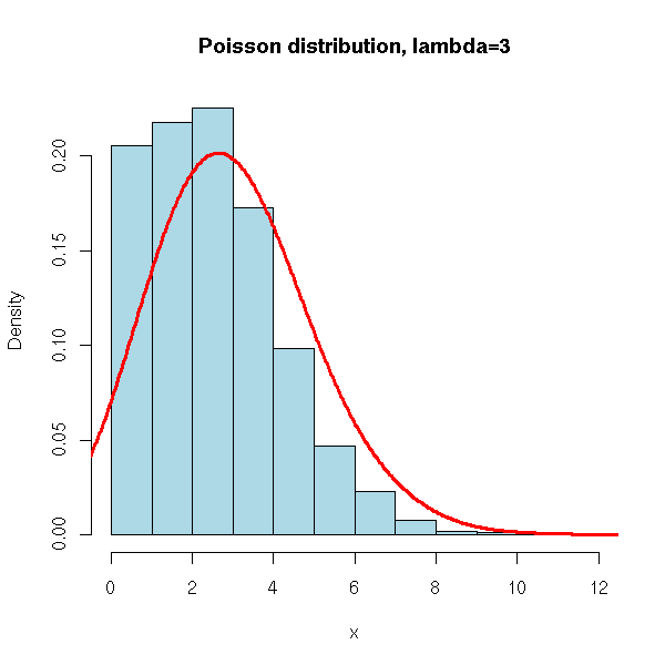
N <- 10000
x <- rpois(N, 5)
hist(x,
     xlim=c(min(x),max(x)), probability=T, nclass=max(x)-min(x)+1,
     col='lightblue',
     main='Poisson distribution, lambda=5')
lines(density(x,bw=1), col='red', lwd=3)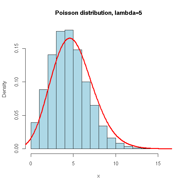
N <- 10000
x <- rpois(N, 20)
hist(x,
     xlim=c(min(x),max(x)), probability=T, nclass=max(x)-min(x)+1,
     col='lightblue',
     main='Poisson distribution, lambda=20')
lines(density(x,bw=1), col='red', lwd=3)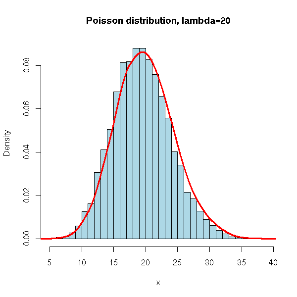
It is the number of trials before a success in a series of Bernoulli events. For instance, if we are interested in the occurrences of 1s and if we get
0 0 0 1 0 1 0 0 1 0 0 1 0
then, we have three trials (0 0 0, at the begining) before a success (the fourth element is "1").
We could simulate it by hand
my.rgeom <- function (N, p) {
  bernoulli <- sample( c(0,1), N, replace=T, prob=c(1-p, p) )
  diff(c(0, which(bernoulli == 1))) - 1
}
hist( my.rgeom(10000, .5), col="light blue",
      main="Geometric distribution" )
but it is easier to use the "rgeom" command.
N <- 10000
x <- rgeom(N, .5)
hist(x,
     xlim=c(min(x),max(x)), probability=T, nclass=max(x)-min(x)+1,
     col='lightblue',
     main='Geometric distribution, p=.5')
lines(density(x,bw=1), col='red', lwd=3)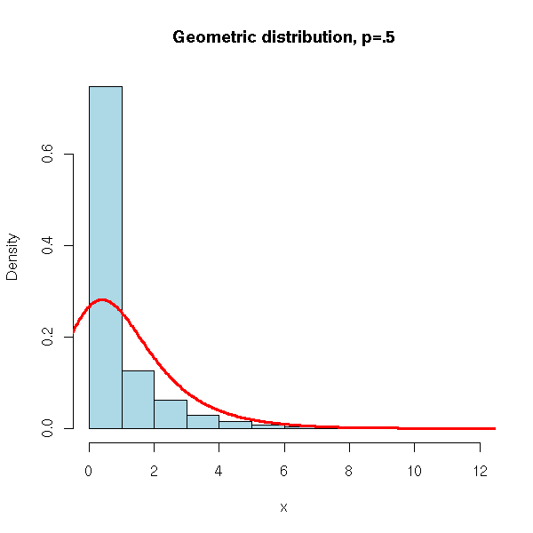
N <- 10000
x <- rgeom(N, .1)
hist(x,
     xlim=c(min(x),max(x)), probability=T, nclass=max(x)-min(x)+1,
     col='lightblue',
     main='Geometric distribution, p=.1')
lines(density(x,bw=1), col='red', lwd=3)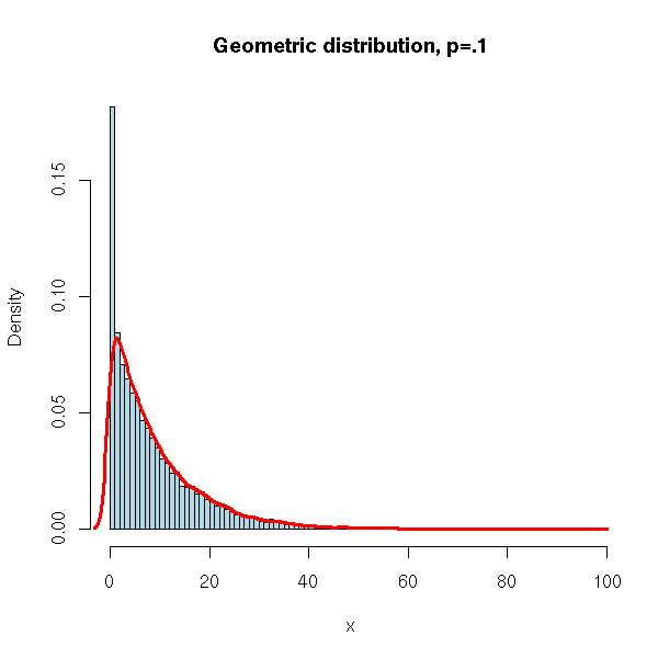
N <- 10000
x <- rgeom(N, .01)
hist(x,
     xlim=c(min(x),max(x)), probability=T, nclass=20,
     col='lightblue',
     main='Geometric distribution, p=.01')
lines(density(x), col='red', lwd=3)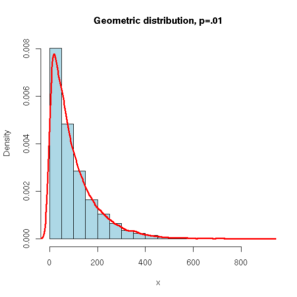
It is the distribution of the number of failures before k successes in a series of Bernoulli events.
We could simulate it by hand (exercice left to the reader). but it is easier to resort to the "rnbinom" function.
N <- 100000
x <- rnbinom(N, 10, .25)
hist(x,
     xlim=c(min(x),max(x)), probability=T, nclass=max(x)-min(x)+1,
     col='lightblue',
     main='Negative binomial distribution, n=10, p=.25')
lines(density(x,bw=1), col='red', lwd=3)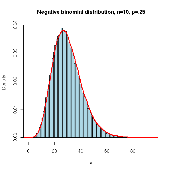
N <- 10000
x <- rnbinom(N, 10, .5)
hist(x,
     xlim=c(min(x),max(x)), probability=T, nclass=max(x)-min(x)+1,
     col='lightblue',
     main='negative binomial distribution, n=10, p=.5')
lines(density(x,bw=1), col='red', lwd=3)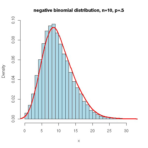
N <- 10000
x <- rnbinom(N, 10, .75)
hist(x,
     xlim=c(min(x),max(x)), probability=T, nclass=max(x)-min(x)+1,
     col='lightblue',
     main='negative binomial distribution, n=10, p=.75')
lines(density(x,bw=1), col='red', lwd=3)
It is the analogue of the binomial distribution but, this time, the events have several possible outcomes.
P( (X1,X2,...,Xn)=(k1,k2,...,kn) ) = m! p1^k1 ... pn^kn / (k1! ... kn!)
We can simulate it as follows, still with the "sample" function.
n <- 5
N <- 100
p <- c(.2,.5,.1,.1,.1)
x <- factor(sample(1:n, N, replace=T, prob=p), levels=1:n)
table(x)
We get:
x
 1  2  3  4  5
19 47 13  7 14
The most important continuous probability distributions are the gaussian, exponential and uniform distributions.
Here, "uniform" means "evenly distributed in a given interval". This is the distribution we expect when we want to "take a number at random in the interval [0,1]".
We can simulate this distribution with the "runif" function.
> round(runif(20), digits=4)
 [1] 0.6187 0.4653 0.0806 0.5425 0.4418 0.4485 0.4685 0.4461 0.9195 0.6127
[11] 0.9132 0.8607 0.1341 0.3795 0.8608 0.9100 0.1545 0.7401 0.2990 0.8714
We can see it as an analogue of the Poisson distribution. Actually, the time between two event in a Poisson process (intuitively: the time between two rare events) follows an exponential distribution. For instance, the time between two radioactive disintegrations.
curve(dexp(x), xlim=c(0,10), col='red', lwd=3,
      main='Exponential Probability Distribution Function')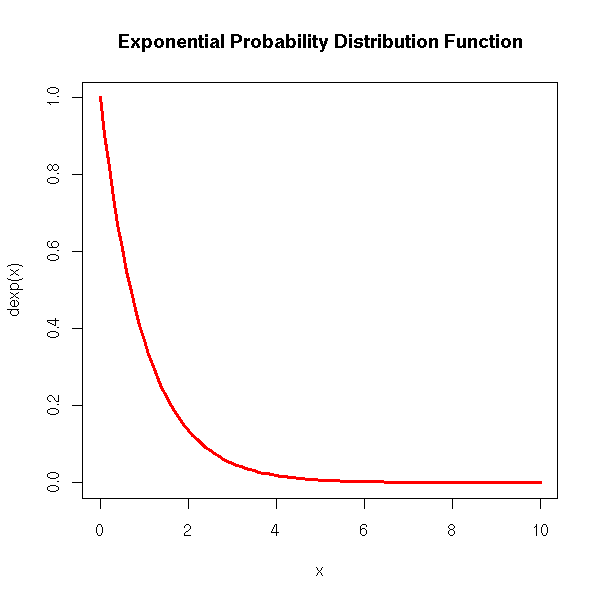
n <- 1000
x <- rexp(n)
hist(x, probability=T,
     col='light blue', main='Exponential Distribution')
lines(density(x), col='red', lwd=3)
curve(dexp(x), xlim=c(0,10), col='red', lwd=3, lty=2,
      add=T)
This is the famous "bell-shaped" distribution.
More precisely, the central limit theorem states that if X1, X2, ... X3 are independant identically distributed random varaibles with expectation m avd variance s^2, then
 (X1+X2+...+Xn) - nm
---------------------
      sqrt(n) s
converges in law to a gaussian distribution when n tends to infinity.
in other words, the empirical means
X1+...Xn
--------
    n
is "close to" a gaussian distribution of expectation m and standard deviation s/sqrt(n).
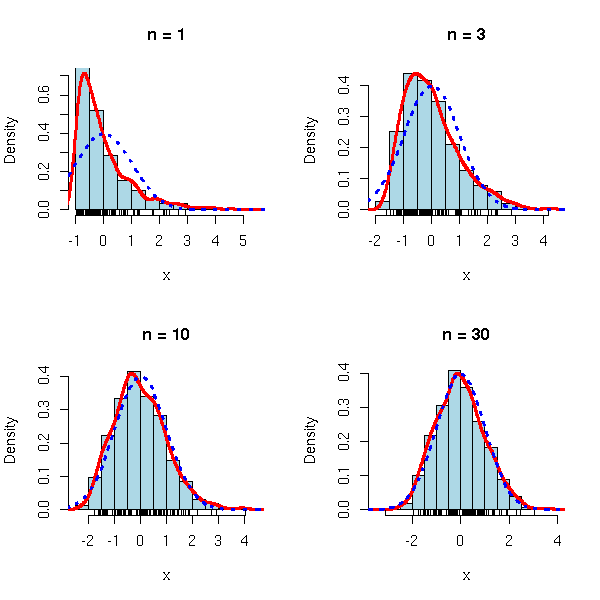
This explains the omnipresence of the gaussian law: when you repeat an experiment a large number of times, the average result (almost) follows a gaussian distribution.
limite.centrale <- function (r=runif, m=.5, s=1/sqrt(12), n=c(1,3,10,30), N=1000) {
  for (i in n) {
    x <- matrix(r(i*N),nc=i)
    x <- ( apply(x, 1, sum) - i*m )/(sqrt(i)*s)
    hist(x, col='light blue', probability=T, main=paste("n =",i),
         ylim=c(0,max(.4, density(x)$y)))
    lines(density(x), col='red', lwd=3)
    curve(dnorm(x), col='blue', lwd=3, lty=3, add=T)
    if( N>100 ) {
      rug(sample(x,100))
    } else {
      rug(x)
    }
  }
}
op <- par(mfrow=c(2,2))
limite.centrale()
par(op)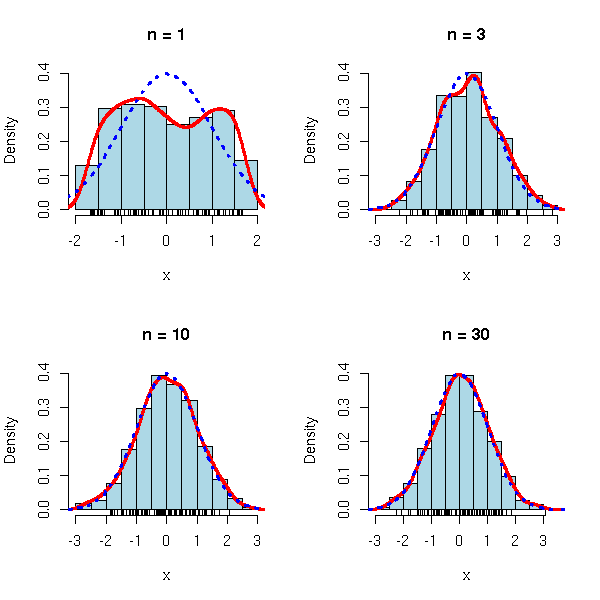
op <- par(mfrow=c(2,2))
limite.centrale(rexp, m=1, s=1)
par(op)

op <- par(mfrow=c(2,2))
limite.centrale(rexp, m=1, s=1)
par(op)
op <- par(mfrow=c(2,2))
limite.centrale(function (n) { rnorm(n, sample(c(-3,3),n,replace=T)) },
                m=0, s=sqrt(10), n=c(1,2,3,10))
par(op)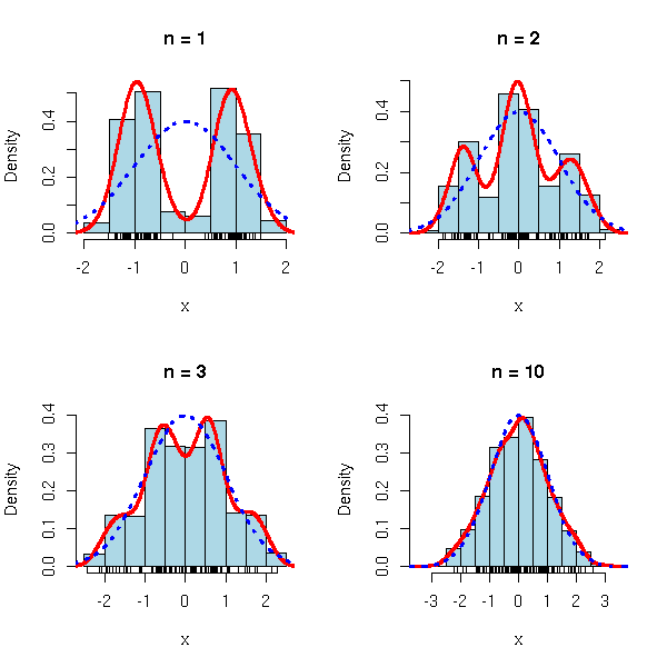
Exercise: dra a plot, similar to the one above, but with the theoretical probability densities.
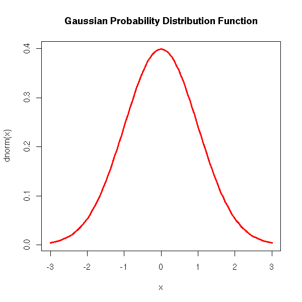
For the formula-savvy reader, the gaussian probability density function is
f(x) = exp( -x^2/2 ) / sqrt( 2 pi )
In R:
curve(dnorm(x), xlim=c(-3,3), col='red', lwd=3)
title(main='Gaussian Probability Distribution Function')
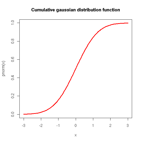
The cumulative density (i.e., the integral of the density):
curve(pnorm(x), xlim=c(-3,3), col='red', lwd=3)
title(main='Cumulative gaussian distribution function')
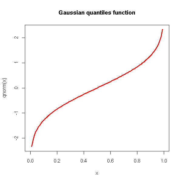
The quantiles (i.e., the inverse of the cumulative density):
curve(qnorm(x), xlim=c(0,1), col='red', lwd=3)
title(main='Gaussian quantiles function')
And, of course, we have an "rnorm" function for simulations.
n <- 1000
x <- rnorm(n)
hist(x, probability=T, col='light blue', main='Gaussian Distribution')
lines(density(x), col='red', lwd=3)
curve(dnorm(x), add=T, col='red', lty=2, lwd=3)
legend(par('usr')[2], par('usr')[4], xjust=1,
       c('sample density', 'theoretical density'),
       lwd=2, lty=c(1,2),
       col='red')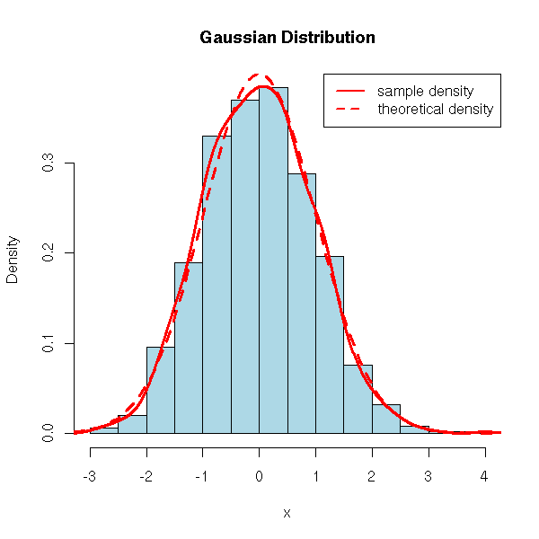
In the discussion above, we had assumed the mean was mu=0 and the standard deviation sigma=1 (the "standard gaussian" distribution): to get the general case, we just apply an affine transformation:
f(x) = exp( -( (x-mu) / sigma )^2 /2 ) / sqrt( 2 pi sigma )
The gaussian distribution is sometimes called the "normal" distribution -- I shall try to avoid this word, because in some situations, the distribution we would like to observe (the one we would like to call "normal") is not the gaussian one.
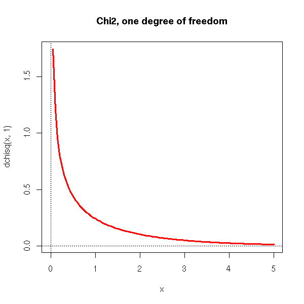
This is the distribution of X^2, if the random variable X follows a standard gaussian distribution.
curve(dchisq(x,1), xlim=c(0,5), col='red', lwd=3)
abline(h=0,lty=3)
abline(v=0,lty=3)
title(main="Chi2, one degree of freedom")
This is the probability distribution of X1^2+...+Xn^2, where the random variables X1, X2, ..., Xn are independant standard gaussian.
We meet this distribution in statistics, when do computations that require the population variance, without knowing this variance: we replace it by the variance of the sample.
We shall discuss this in more depth when we tackle estimators and statistical tests.
curve(dchisq(x,1), xlim=c(0,10), ylim=c(0,.6), col='red', lwd=3)
curve(dchisq(x,2), add=T, col='green', lwd=3)
curve(dchisq(x,3), add=T, col='blue', lwd=3)
curve(dchisq(x,5), add=T, col='orange', lwd=3)
abline(h=0,lty=3)
abline(v=0,lty=3)
legend(par('usr')[2], par('usr')[4], xjust=1,
       c('df=1', 'df=2', 'df=3', 'df=5'),
       lwd=3,
       lty=1,
       col=c('red', 'green', 'blue', 'orange')
      )
title(main='Chi^2 Distributions')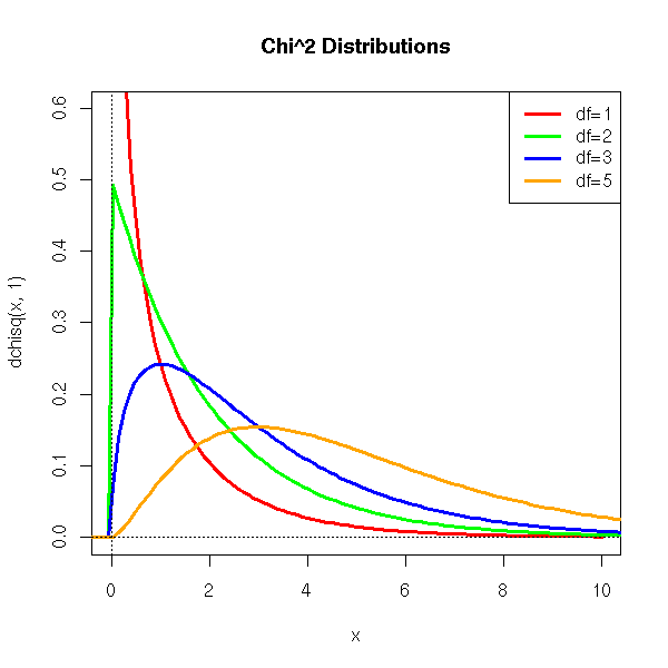
If X1, X2, X3,... are independant identically distributed gaussian random variables of expectation mu and standard deviation sigma, then
  X1 + X2 + ... + Xn
 --------------------  -  mu
          n
-----------------------------
          sigma
        ---------
         sqrt(n)
follows a gaussian law. But if we replace the standard deviation by the sample standard deviation (i.e., an estimator of the population standard deviation), this quantity no longer follows a gaussian distribution but a Student T distribution with (n-1) degrees of freedom.
curve( dt(x,1), xlim=c(-3,3), ylim=c(0,.4), col='red', lwd=2 )
curve( dt(x,2), add=T, col='blue', lwd=2 )
curve( dt(x,5), add=T, col='green', lwd=2 )
curve( dt(x,10), add=T, col='orange', lwd=2 )
curve( dnorm(x), add=T, lwd=3, lty=3 )
title(main="Student T distributions")
legend(par('usr')[2], par('usr')[4], xjust=1,
       c('df=1', 'df=2', 'df=5', 'df=10', 'Gaussian distribution'),
       lwd=c(2,2,2,2,2),
       lty=c(1,1,1,1,3),
       col=c('red', 'blue', 'green', 'orange', par("fg")))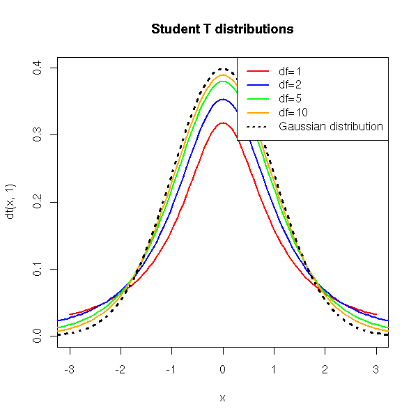
If X1, X2, ... Xn and Y1, Y2,... Ym are independant identically distributes gaussian random variables, then
  X1^2 + X2^2 + ... + Xn^2
 --------------------------
            n
----------------------------
  Y1^2 + Y2^2 + ... + Ym^2
 --------------------------
            m
follows an F distribution, with n and m degrees of freedom. This, it is the distribution of a quotient of independant Chi2 variables, each divided by its degree of freedom.
We shall meet this distribution when we compare variances (for instance, in Anova (ANalysis Of VAriance) or in statistical tests).
curve(df(x,1,1), xlim=c(0,2), ylim=c(0,.8), lty=2)
curve(df(x,3,1), add=T)
curve(df(x,6,1), add=T, lwd=3)
curve(df(x,3,3), add=T, col='red')
curve(df(x,6,3), add=T, lwd=3, col='red')
curve(df(x,3,6), add=T, col='blue')
curve(df(x,6,6), add=T, lwd=3, col='blue')
title(main="Fisher's F")
legend(par('usr')[2], par('usr')[4], xjust=1,
       c('df=(1,1)', 'df=(3,1)', 'df=(6,1)',
         'df=(3,3)', 'df=(6,3)',
         'df=(3,6)', 'df=(6,6)'),
       lwd=c(1,1,3,1,3,1,3),
       lty=c(2,1,1,1,1,1,1),
       col=c(par("fg"), par("fg"), par("fg"), 'red', 'red', 'blue', 'blue'))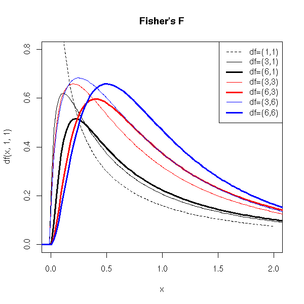
Quite often, the variables we meet in the real world have positive values: with a truly gaussian variable, this is not possible -- we know that our variable is not gaussian. Instead, we can look if ots logarithm is gaussian -- in other words, if our variable is the exponential of a gaussian variable.
curve(dlnorm(x), xlim=c(-.2,5), lwd=3,
      main="Log-normal distribution")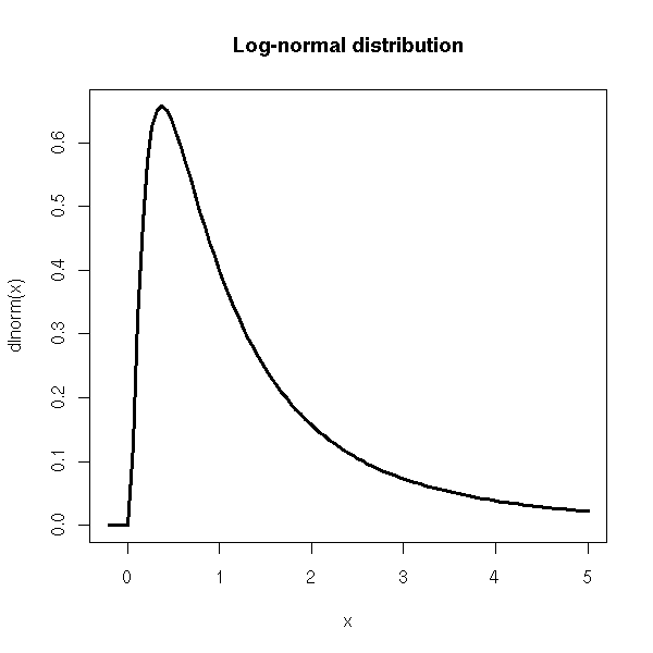
This is an example of a pathologically dispersed distribution: its variance is infinite.
It is sometimes called the bowman's distribution: a blindfolded bowman, in front of an infinite wall shoots arrows in random directions. The distribution of the arrow impacts on the wall is a Cauchy distribution.
N <- 100                         # Number of arrows
alpha <- runif(N, -pi/2, pi/2)   # Direction of the arrow
x <- tan(alpha)                  # Arrow impact
plot.new()
plot.window(xlim=c(-5, 5), ylim=c(-1.1, 2))
segments( 0, -1,     # Position of the Bowman
          x, 0   )   # Impact
d <- density(x)
lines(d$x, 5*d$y, col="red", lwd=3 )
box()
abline(h=0)
title(main="The bowman's distribution (Cauchy)")
# Exercise: turn this into an animation...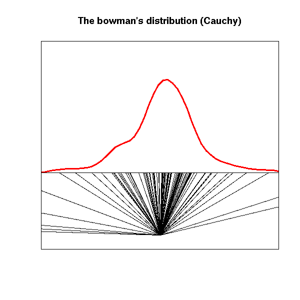
N <- 10000
x <- tan(runif(N, -pi/2, pi/2))
xlim <- qcauchy(2/N)
xlim <- c(xlim, -xlim)
plot(qcauchy(ppoints(N)),  sort(x),
     xlim=xlim, ylim=xlim,
     main="The bowman's distribution and Cauchy's")
It is also a limiting case of the Student T distribution, with 1 degree of freedom.
curve(dcauchy(x),xlim=c(-5,5), ylim=c(0,.5), lwd=3)
curve(dnorm(x), add=T, col='red', lty=2)
legend(par('usr')[2], par('usr')[4], xjust=1,
       c('Cauchy distribution', 'Gaussian distribution'),
       lwd=c(3,1),
       lty=c(1,2),
       col=c(par("fg"), 'red'))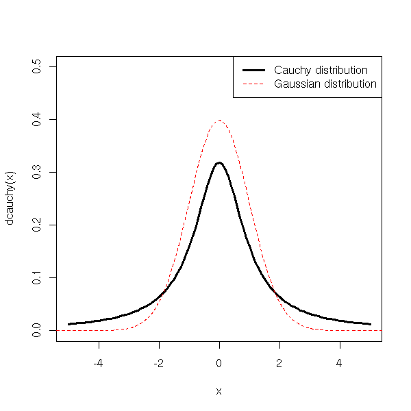
Distributions with "more" extreme values than a gaussian distribution are called "fat-tailed" distributions: the Student T distribution or the Cauchy distribution are fat-tailed.
Brownian motion built with a fat-tailed distribution (sometimes called "Levy flight") is sometimes used to model epidemics or foraging animals: locally, it looks like plain brownian motion, but from time to time, there is a large jump and the process (or the animal) starts to explore another part of the plane.
N <- 100
x <- cumsum(rnorm(N))
y <- cumsum(rnorm(N))
plot(x, y,
     type = "o", pch = 16, lwd = 2,
     xlab = "", ylab = "",
     axes = FALSE,
     main = "Brownian Motion")
box()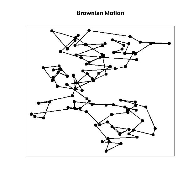
set.seed(1)
x <- cumsum(rt(N, df=2))
y <- cumsum(rt(N, df=2))
plot(x, y,
     type = "o", pch = 16, lwd = 2,
     xlab = "", ylab = "",
     axes = FALSE,
     main = "Levy flight")
box()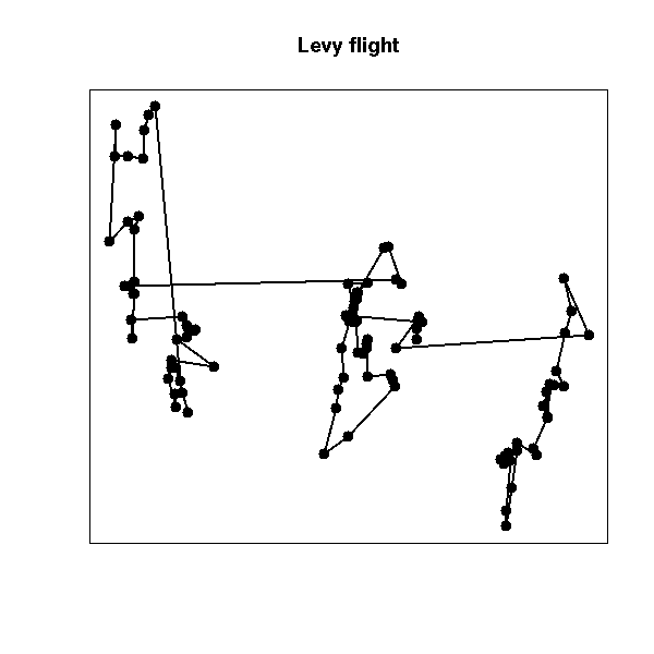
When modeling data, you can often faithfully model a fat-tailed distribution as a mixture of gaussians: you assume the data does not come from a single, gaussian source, but from several -- say, the correct data and measuring errors -- or several data sources, different but all relevant.
N <- 10000
m <- c(-2,0,2)    # Means
p <- c(.3,.4,.3)  # Probabilities
s <- c(1, 1, 1)   # Standard deviations
x <- cbind( rnorm(N, m[1], s[1]),
            rnorm(N, m[2], s[2]),
            rnorm(N, m[3], s[3]) )
a <- sample(1:3, N, prob=p, replace=TRUE)
y <- x[ 1:N + N*(a-1) ]

qqnorm(y,
       main="Gaussian QQ-plot of a mixture of gaussians")
qqline(y, col="red", lwd=3)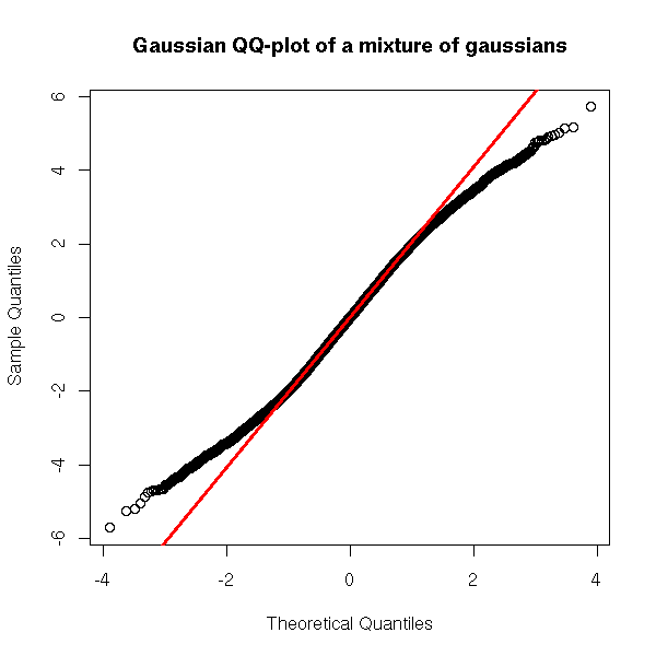
hist(y, col="light blue", probability=TRUE,
     ylim=c(0,.25),
     main="Mixture of gaussians")
curve(dnorm(x, mean=mean(y), sd=sd(y)),
      add=TRUE, col="red", lwd=3, lty=2)
lines(density(x), col="red", lwd=3)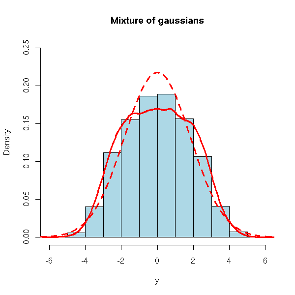
curve( p[2] * dnorm(x, mean=m[2], sd=s[2]),
       col = "green", lwd = 3,
       xlim = c(-5,5),
       main = "The three gaussian distributions in our mixture",
       xlab = "", ylab = "")
curve( p[1] * dnorm(x, mean=m[1], sd=s[1]),
       col="red", lwd=3, add=TRUE)
curve( p[3] * dnorm(x, mean=m[3], sd=s[3]),
       col="blue", lwd=3, add=TRUE)
n <- 200
x <- seq(-5, 5, length=n)
y3 <- p[1] * dnorm(x, mean=m[1], sd=s[1]) +
      p[2] * dnorm(x, mean=m[2], sd=s[2]) +
      p[3] * dnorm(x, mean=m[3], sd=s[3])
y2 <- p[1] * dnorm(x, mean=m[1], sd=s[1]) +
      p[2] * dnorm(x, mean=m[2], sd=s[2])
y1 <- p[1] * dnorm(x, mean=m[1], sd=s[1])
plot.new()
plot.window(xlim=range(x), ylim=range(0,y1,y2,y3))
polygon(c(x[1],x,x[n]), c(0,y3,0), col="blue",  border=NA)
polygon(c(x[1],x,x[n]), c(0,y2,0), col="green", border=NA)
polygon(c(x[1],x,x[n]), c(0,y1,0), col="red",   border=NA)
lines(x, y1, lwd=3)
lines(x, y2, lwd=3)
lines(x, y3, lwd=3)
box()
axis(1)
title("Mixture of gaussians")
TODO:
mclust
norm1mix

TODO: Model real data as a mixture of gaussians.
      Compare with a model of the data as a gaussian,
      Student T or Cauchy distribution (with qqplots)
One usually defines mixtures using the distribution functions. Instead, one could define them using the quantile functions. For instance, a gaussian-polynomial quantile mixture has a quantile function of the form
q(p) = qnorm(p) + a * p + b * p^2 + x * p^3.
(Beware, not any value of a, b anc c will do: the quantile function has to be increasing!)
One could similarly define a Cauchy-polynomial quantile mixture.
q <- function (p, a=1, b=0, c=0, d=0) {
  a * qnorm(p) + b + c * p + d * p^2
}
N <- 10000
x <- runif(N)
op <- par(mfrow=c(2,3))
for (a in c(-2,2)) {
  y <- q(x, 1, -a/2, a)
  hist(y,
       xlab = "",
       main = "Gaussian-polynomial quantile mixture",
       col = "light blue",
       probability = TRUE)
  curve(q(x, 1, -a/2, a),
        lwd = 3,
        xlim = c(0,1), ylim = c(-3,3),
        xlab = "",
        main = "Quantile function")
  abline(h = 0,
         v = c(0, .5, 1),
         lty = 3)
  curve(qnorm(x), lty = 2, add = TRUE)
  qqnorm(y)
  qqline(y, col="red")
}
par(op)
Those distributions can be used as a generalization of a classical distribution (gaussian, Cauchy, etc.), together with L-moments or trimmed L-moments (TL-moments).
TODO: URL
Estimation of quantile mixtures via L-moments and trimmed L-moments
J. Karvanen (2005)
See also the lmomco package.
library(help=lmomco)
AN edgeworth expansion is an approximation of a univariate distribution, e.g., so that the first moments (mean, standard deviation, skewness, kurtosis) be correct.
Here is an application to option pricing with non-log-normal underlying:
M. Rubinstein, Edgeworth binomial tree
http://www.haas.berkeley.edu/finance/WP/rpf275.pdf
The Cauchy distribution is (together with the gaussian distribution) a member of the family of "stable distributions" (also called "Levy distributions" or "Levy-stable distributions" or "Pareto-Levy distributions"): this means that a sum of Cauchy variables is still a Cauchy varible. Thus, one may expect to find the Cauchy distribution, or more generally stable distributions, from time to time, in natural phenomena.
More precisely, stable distributions satisfy a limit theorem similar to the central limit theorem. The central limit theorem states that, under some often satisfied conditions, if X1, X2, ..., Xn are independant identically distributed random variables, then their average (X1+...+Xn)/n "converges" (in some sense) to a gaussian distribution. But in those "often satisfied" conditions, we require that the distribution have a variance. What if the distribution is so fat-tailed that the variance is infinite? There is a more general limit theorem, with more general hypotheses: the everage (X1+...+Xn)/n converges towards a stable distribution.
?StableDistribution

library(fBasics)
# alpha=2 is the gaussian distribution
# alpha<2 distributions have fat tails
x <- rsymstb(10000, alpha=1.5)
y <- x[ abs(x) < 10 ]
hist(y,
     ylim = c(0, .4),
     col = "light blue",
     probability = TRUE,
     xlab = "", ylab = "",
     main = "A stable distribution (alpha=1.5)")
lines(density(y), col = "red", lwd = 3)
curve(dnorm(x),   col = "red", lwd = 3, lty=2,
                  add = TRUE)
For more on the subject, check:
http://academic2.american.edu/~jpnolan/stable/chap1.pdf
The Levy distribution is one of the stable distributions. It is fat-tailed, asymetric and its expectation is infinite.
It is obtained, for instance, as the hitting times of a brownian motion.
set.seed(1)
N <- 1e7
x <- sample(c(-1,+1), N, replace = TRUE)
x <- cumsum(x)          # Random walk
x <- diff(which(x==0))  # Time to go back to zero
r <- density(x[x<100])
plot(r$x, log(r$y),
     xlim = c(0,20),
     ylim = c(-6,0),
     type = "l",
     xlab = "Hitting time",
     ylab = "log(density)",
     main = "(Discretized) Levy distribution")
v <- r$x[ which.max(r$y) ]  # Mode
abline(v = v, lty=3, lwd=3)
curve( dnorm(x, mean = v, sd = 1, log = TRUE) -
       dnorm(0,sd=1,log=T) + log(max(r$y)) ,
       add = TRUE, col = "blue", lwd = 3, lty = 2 )
The Weibull distribution is a generalization of the exponential distribution in which the "decrease rate" (the correct word is "hazard rate" -- more about this when we tackle survival analysis) is not constant. It is used to model the lifetime (time without a failure) of a machine (this "decrease rate", i.e., the probability a problem occurs, grows with the age of the machine).
The density is of the form exp(-a t^b).
curve(dexp(x), xlim=c(0,3), ylim=c(0,2))
curve(dweibull(x,1), lty=3, lwd=3, add=T)
curve(dweibull(x,2), col='red', add=T)
curve(dweibull(x,.8), col='blue', add=T)
title(main="Weibull Probability Distribution Function")
legend(par('usr')[2], par('usr')[4], xjust=1,
       c('Exponential', 'Weibull, shape=1',
         'Weibull, shape=2', 'Weibull, shape=.8'),
       lwd=c(1,3,1,1),
       lty=c(1,3,1,1),
       col=c(par("fg"), par("fg"), 'red', 'blue'))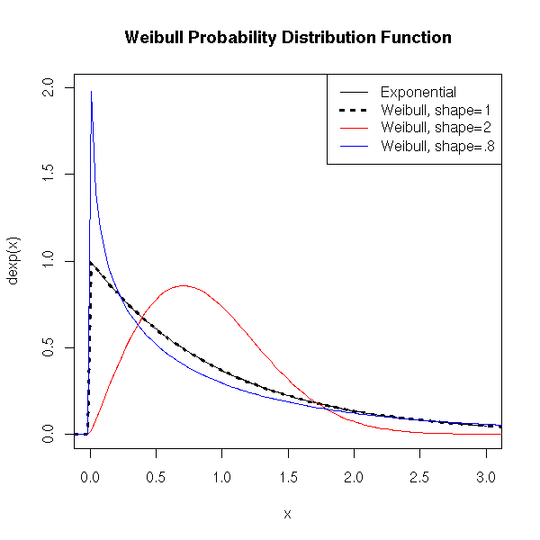
This is the distribution of a sum of independant exponential random variables. As such, it is a generalization of the exponential distribution, use to model lifetimes (for instance, a reliable machine that would have to undergo three successive problems to stop functionning, each problem being described by an exponential law).
The arrival times in a Poisson process are Gamma-distributed.
curve( dgamma(x,1,1), xlim=c(0,5) )
curve( dgamma(x,2,1), add=T, col='red' )
curve( dgamma(x,3,1), add=T, col='green' )
curve( dgamma(x,4,1), add=T, col='blue' )
curve( dgamma(x,5,1), add=T, col='orange' )
title(main="Gamma probability distribution function")
legend(par('usr')[2], par('usr')[4], xjust=1,
       c('k=1 (Exponential distribution)', 'k=2', 'k=3', 'k=4', 'k=5'),
       lwd=1, lty=1,
       col=c(par('fg'), 'red', 'green', 'blue', 'orange') )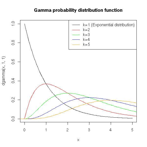
n <- 500
x1 <- rexp(n,17)
x2 <- rexp(n,17)
x3 <- rexp(n,17)
x <- x1 + x2 + x3
# Simpler, but less readable:
# k <- 3
# x <- drop(apply( matrix( rexp(n*k,17), nr=n, nc=k ), 1, sum))
y <- qgamma(ppoints(n),3,17)
plot( sort(x) ~ sort(y), log='xy' )
abline(0,1, col='red')
title("Comparision: gamma distribution and sum of exponential r.v.")
See also:
http://www.math.uah.edu/statold/special/special3.html
Here is the definition you will find in most books (it is not enlightening, I shall therefore give more intuitive definitions in a few moments): If X and T are independant random variables, following Gamma distributions of parameters (a,r) and (b,r), then X/(X+Y) is distributed according to a Beta distribution of parameters (a,b).
curve( dbeta(x,1,1), xlim=c(0,1), ylim=c(0,4) )
curve( dbeta(x,2,1), add=T, col='red' )
curve( dbeta(x,3,1), add=T, col='green' )
curve( dbeta(x,4,1), add=T, col='blue' )
curve( dbeta(x,2,2), add=T, lty=2, lwd=2, col='red' )
curve( dbeta(x,3,2), add=T, lty=2, lwd=2, col='green' )
curve( dbeta(x,4,2), add=T, lty=2, lwd=2, col='blue' )
curve( dbeta(x,2,3), add=T, lty=3, lwd=3, col='red' )
curve( dbeta(x,3,3), add=T, lty=3, lwd=3, col='green' )
curve( dbeta(x,4,3), add=T, lty=3, lwd=3, col='blue' )
title(main="Beta distribution")
legend(par('usr')[1], par('usr')[4], xjust=0,
       c('(1,1)', '(2,1)', '(3,1)', '(4,1)',
         '(2,2)', '(3,2)', '(4,2)',
         '(2,3)', '(3,3)', '(4,3)' ),
       lwd=1, #c(1,1,1,1, 2,2,2, 3,3,3),
       lty=c(1,1,1,1, 2,2,2, 3,3,3),
       col=c(par('fg'), 'red', 'green', 'blue',
             'red', 'green', 'blue',
             'red', 'green', 'blue' ))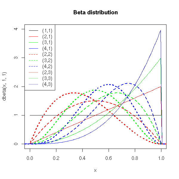
If X1,X2,...,Xn are independant random variables, uniformly distributed in [0,1], then max(X1,X2,...,Xn) is distributed according to a Beta distribution of parameters (n,1).
N <- 500
n <- 5
y <- drop(apply( matrix( runif(n*N), nr=N, nc=n), 1, max ))
x <- qbeta(ppoints(N), n, 1)
plot( sort(y) ~ x )
abline(0,1, col='red')
title("Order statistic and Beta distribution")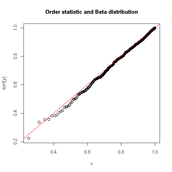
The orther order statistics (the k-th largest element of X1,X2,...,Xn) follow other Beta distributions.
N <- 500
n <- 5
k <- 3
y <- drop(apply( matrix( runif(n*N), nr=n, nc=N), 2, sort )[n-k,])
x <- qbeta(ppoints(N), n-k, k+1) # Exercice: Where do those
                                 # coefficients come from?
plot( sort(y) ~ x )
abline(0,1, col='red')
title("Order statistics and Beta distribution")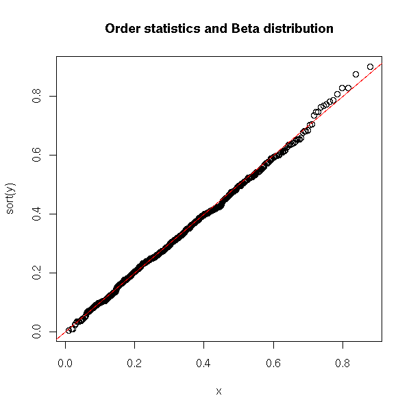
# I admit it: I found the coefficients above by trial-and-error...
op <- par(mfrow=c(5,5), mar=c(0,0,0,0) )
for (i in 1:5) {
  for (j in 1:5) {
    plot( sort(y) ~ qbeta(ppoints(N), j, i), xlab='', ylab='', axes=F )
    abline(0,1, col='red')
    box()
    text( (par('usr')[1]+par('usr')[2])/2,
          (par('usr')[3]+par('usr')[4])/2,
          paste(j,i),
          cex=3, col='blue' )
  }
}
par(op)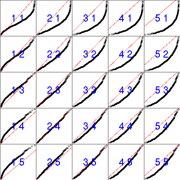
See also:
http://www.math.uah.edu/statold/special/special9.html
Here is another, bayesian, motivation for the Beta distribution. "Bayesian" means that, when we are interested in some parameter (say, the probability of getting "tails" when tossing a coin), we do not want to get a single precise value -- we are sure it would be wrong --, we want a whole distribution, e.g., "the probability of getting tails seems to be taken from a gaussian distribution of mean 0.4 and standard deviation 0.1". (Here, you should stand up and scream: it cannot be a gaussian distribution, it must be some distribution whose values are limited to [0,1]!)
Let us toss a coin (it is funnier if it has been tampered with; if you cannot find one, you can use a drawing pin instead) and try to find the probability of getting tails. We do not know anything, a priori, about this probability. If we wanted to give a number for it, we would give "0.5", but it is more precise to give a distribution: the "prior probability" is described by a uniform distribution in [0,1]. It means that we do not know anything, that we do not have any information that could suggest a preference for some probability. If we toss the coin (drawing pin) 10 times and observe 7 tails and 3 heads, we have more information and we can uptate our probability distribution for p: it is proportionnal to
p^7 * (1-p)^3.
This is a Beta(8,4) distribution.
curve(dbeta(x,8,4),xlim=c(0,1))
title(main="posterior distrobution of p")

You can do the experiment in two steps: you start with a uniform prior, you toss a few coins/drawing pins, you get a beta posterior; if you toss a few more coins, you can transform this beta distribution (the beta posterior of the first series of tosses is the prior of the second series of tosses) into another beta distribution. That is why one often uses the beta distribution as a prior distribution, when one uses bayesian methods to estimate probabilities (or any bounded quantity).
In a more simple and intuitive way, one can use a beta distribution to model a continuous distribution in the interval [0,1], with a peak, more or less important, more or less skewed.
As a result, you may want to use this distribution to model any bounded quantity.
curve(dbeta(x,10,10), xlim=c(0,1), lwd=3)
curve(dbeta(x,1,1), add=T, col='red', lwd=3)
curve(dbeta(x,2,2), add=T, col='green', lwd=3)
curve(dbeta(x,5,2), add=T, col='blue',lwd=3)
curve(dbeta(x,.1,.5), add=T, col='orange')
legend(par('usr')[2], par('usr')[4], xjust=1,
       c('B(10,10)', 'B(1,1)', 'B(2,2)', 'B(5,2)', 'B(.1,.5)'),
       lwd=c(3,3,3,3,1), lty=1,
       col=c(par('fg'),'red','green','blue','orange'))
title("A few beta probability distributions")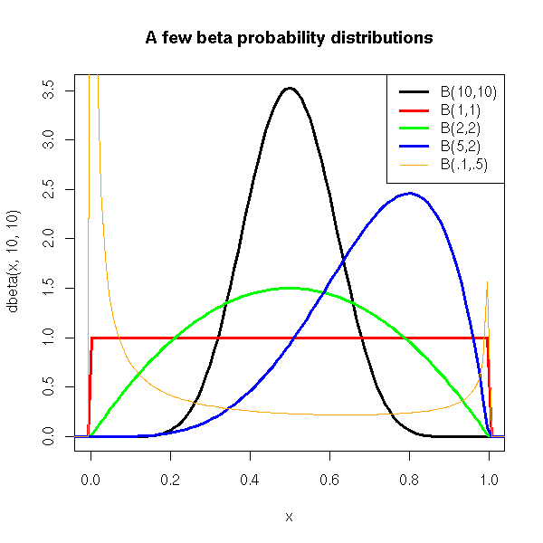
Here is another presentation of this bayesian motivation for the Beta distribution, with no bayesian ideas but "just" maximum likelihood. The situation is the same: we toss a coin or a drawing pin and we look on which side it falls. We call p the probability of getting "tails". We got 7 tails and 3 heads. We can see 7 as the value of a binomial variable of parameters (10,p). The probability of observing 7 tails and 3 heads given p is
L(p) = p^7 * (1-p)^3.
This probability is called "likelihood" (in more general terms, the "likelihood" of a parameter p is the probability of observing the results we actually observed given the value of p -- it is a function of p, which we usually use to compyte the "most probable value of p", i.e., the value pf p that maximizes the likelihood). As before, it is proportional to the density of a Beta distribution.
We say that the binomial and the beta distribution are conjugated: their density is given by the same formula by interverting the role of the parameter and the variable.
This is a multidimensionnal generalization of the beta distribution, extensively used in bayesian modelling: the Beta distribution can be used to model the distribution of the p paremeter of a binomial random variable; similarly, the Dirichlet distribution can be used to model the distribution of the probabilities used as parameters of a multinomial distribution.
library(gtools)
?rdirichlet

library(bayesm)
?rdirichlet

library(MCMCpack)
?Dirichlet

TODO

If X1,...,Xn are independant Gamma distributions, then
(X1,...,Xn)/(X1+...+Xn) follows a Beta distribution.
Most of the distributions presented here belong to the family of exponential distributions -- they play an important role in some theoretical results, mainly because they are amenable to explicit (closed-formula) computations, but their definition might not be very enlightening:
                         y theta - v(theta)
f(y, theta,phi) = exp ( -------------------- + w(y,phi) )
                              u(phi)
For simulations (especially if you want to know how the algorithm you just developed is "robust", i.e., behaves well with non-gaussian distributions -- or even, with no assumption in the distribution), you can have a look at the Marron--Wand distributions in the nor1mix package.
# Example from the manual
library(nor1mix)
ppos <- which("package:nor1mix" == search())
nms <- ls(pat="^MW.nm", pos = ppos)
nms <- nms[order(as.numeric(substring(nms,6)))]
op <- par(mfrow=c(4,4), mgp = c(1.2, 0.5, 0), tcl = -0.2,
          mar = .1 + c(2,2,2,1), oma = c(0,0,3,0))
for(n in nms) { plot(get(n, pos = ppos)) }
  mtext("The Marron-Wand Densities", outer = TRUE,
        font = 2, cex = 1.6)
par(op)
One can generalize the gaussian distribution in higher dimensions ("multivariate" means that the random variable does not provide us with numbers one at a time, but with points in some vector space -- equivalently, it provides us with n numbers (the coordinates) at a time). Before the definition, let us give a few examples.
For instance, if X1,...,Xn are iid gaussian variables, then (X1,...,Xn) is a multivariate gaussian. But it is a very special case: the resulting cloud of points looks perfectly spherical -- and centered in zero.
If X1,...,Xn are independant gaussian random variables, of different means and variances, then (X1,...,Xn) is a multivariate gaussian. The cloud of points is no longer spherical, it can be elongated, but it will be elongated squashed in directions parallel to the axes -- it is still a very special case.
If X1,...,Xn are gaussian variables, with no restrictions on their means, variances and covariances (they need not be independant), then (X1,...,Xn)
This is actually a definition of the multivariate gaussian variables. A multivariate gaussian random variable is entirely determined by its mean (it is a vector) and its variance-covariance matrix.
Equivalently, one can define multivariate gaussian random variables as variables of the form Y=A+B*X, where A is any vector, B any matrix, X=(X1,...,Xn) and X1,...,Xn are iid standard gaussian random variables.
There used to be ne predefined R function to get a multivariate gaussian sample for a given variance-covariance matrix. But you can roll up your own as follows: we start with independant standard gaussian variables X1, X2, ... and we let
Y1 = a*X1
Y2 = b*X1 + c*X2
Y3 = d*X1 + e*X2 + f*X3
etc.
A "quick" computation shows that
cov(Y) = t(A) %*% A
where
     a 0 0 ...
A =  b c 0
     d e f
     ...
So we "just" have to decompose the desired variance-covariance matrix as a product of a triangular matrix and its transpose: this is the Choleski decomposition.
rmnorm <- function (R, C, mu=rep(0,dim(C)[1])) {
  A <- t(chol(C))
  n <- dim(C)[1]
  t(mu + A %*% matrix(rnorm(R*n),nr=n))
}
C <- matrix(c(2,.5,.5,1),nr=2)
mu <- c(2,1)
y <- rmnorm(1000,C, mu)
cov(y)
plot(y)

abline(h=mu[2], lty=3, lwd=3, col='blue')
abline(v=mu[1], lty=3, lwd=3, col='blue')
e <- eigen(C)
r <- sqrt(e$values)
v <- e$vectors
N <- 100
theta <- seq(0,2*pi, length=N)
x <- mu[1] + r[1]*v[1,1]*cos(theta) +
     r[2]*v[1,2]*sin(theta)
y <- mu[2] + r[1]*v[2,1]*cos(theta) +
     r[2]*v[2,2]*sin(theta)
lines(x,y, lwd=3, col='blue')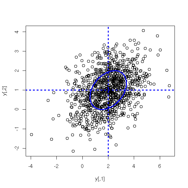
If you want to do computations (and not simulations, as we just did), check the "mvtnorm" package.
library(help=mvtnorm)
Actually, there is already a function to sample from gaussian distributions: "mvrnorm", the the MASS package.
library(MASS)
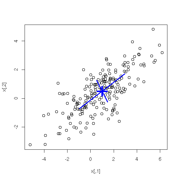
N <- 200
mu <- c(1, .5)
S <- matrix(c(4,2,2,2), nc=2)
x <- mvrnorm(N, mu, S)
plot(x)
# Cloud center
points(mu[1], mu[2], pch=3, cex=3, lwd=5, col="blue")
# Ellipse axes
e <- eigen(S)
a <- mu + sqrt(e$values[1]) * e$vectors[,1]
b <- mu - sqrt(e$values[1]) * e$vectors[,1]
segments(a[1], a[2], b[1], b[2], col="blue", lwd=3)
a <- mu + sqrt(e$values[2]) * e$vectors[,2]
b <- mu - sqrt(e$values[2]) * e$vectors[,2]
segments(a[1], a[2], b[1], b[2], col="blue", lwd=3)
# TODO: Draw the ellipse...
TODO

fitdistr
density estimation
locfit(..., deriv=...) # To get an estimation of the derivative of the density
TODO: there is already a section about EVT slightly below...
I said above that one should not use the word "normal" to speak of the gaussian distribution, because in certain situations, "normal" data are far from gaussian. This is the case in finance (more precisely, in high-frequency (intraday) data), where data are more dispersed than with gaussian distributions. We say that the data have "fat tails".
And the situation is even worse: we are mainly interested in those tails: a high value means high profits (good) or high losses (bad). As those extreme events are more frequent than with a gaussian distribution, as the gaussian distribution fails to describe them properly, and as we wish to focus on them, we should not use the gaussian distribution.
Instead, we can study the truncated distributions:
X | X>a
and
X | X<-a
(Generalized) Extreme Value Distributions are candidate distributions that are hoped to fit more or less closely those truncated distributions.
TODO
evd/doc/guide.pdf
density = exp(-x-exp(-x))

TODO: this should not be in the middle of the
distributions used in survival analysis...
"If things go wrong, how wrong can they go?"
Quite often, when studying voluminous data, we start to assume that they are gaussian. We rarely check this assumption -- if we do, we realize that the gaussian approximation is reasonable for observations close to the mean but completely wrong far from the mean.
The gaussian approximation (with suppression of the most extreme observations) is sufficient if we are only interested in the "usual" behaviour of the data -- but when extreme values play a central role, when we try to understand, fight or use the phenomena that underlie them, this approximation becomes troublesome.
This is the case in risk management: natural disasters (for insurance companies) or stock market crashes are rare events with disastrous consequences -- one cannot afford to improperly evaluate their probabilities and consequences.
Here is an example with stick market data (they were retrieved from Yahoo).
x <- read.table("SUNW.csv", header=T, sep=",")
x <- x$Close
x <- diff(log(x))   # Compute the returns
qqnorm(x, main="Normality of stock returns (15 years)")
qqline(x, col='red')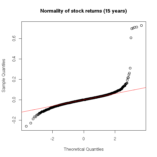
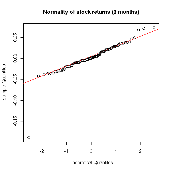
Actually, on a short period, monthly returns are almost normal (the problem is even worse for high freauency (intraday) data).
qqnorm(x[1:90], main="Normality of stock returns (3 months)")
qqline(x[1:90], col='red')
One can graphically compare the sample probability distribution function with that of a gaussian distribution.
plot(density(x), main="Stock returns density vs normal density")
m <- mean(x)
s <- sd(x)
curve( dnorm(x, m, s), col='red', add=T)
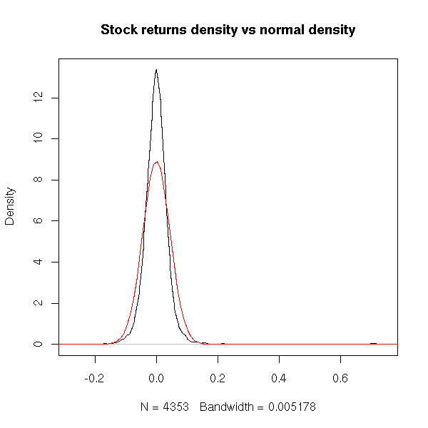
It is clearer on a logarithmic scale.
plot(density(x), log='y', main="Stock returns density vs normal density")
curve( dnorm(x, m, s), col='red', add=T)

plot(density(x), log='y', ylim=c(1e-1,1.5e1), xlim=c(-.2,.2),
     main="Stock returns density vs normal density (detail)")
curve( dnorm(x, m, s), col='red', add=T)
We see that, indeed, the sample distribution has a sharper peak than the normal one -- and is is straiter (on our logarithmic scale): it almost looks like two ligne segments.
Conclusion: in real data, extreme values may be more frequent that in gaussian data.
In risk management, we classically compute three quantities to measure the risk of rare events.
The Value at Risk (VaR) is the alpha-% quantile of the Profits and Losses (P&L) distribution, which we assume normal.
For internal risk control purposes, most of the financial
firms compute a 5% VaR over a one-day holding period. The
Basle accord proposed that VaR for the next 10 days and
p = 1%, based on a historical observation period of at least
1 year (220 days) of data, should be computed and then
multiplied by the `safety factor' 3. The safety factor was
introduced because the normal hypothesis for the profit
and loss distribution is widely recognized as unrealistic.
The Expected Shortfall (ES), or tail conditionnal expectation, is the expectation of the P&L given that it exceeds the VaR.
ES(alpha) = E[ X | X > VaR(alpha) ]
One may consider a third quantity: the n-day k-th return level is the 1/k-quantile of Max(X1,...,Xn), i.e., in one case out of k, the maximum loss in an n-day period will exceed R(n,k).
These two quantities are studied in "Extreme Value Theory" -- indeed, it is not a simgle theory but two:
GEV: Study of Max(X1,...,Xn) (for n large)
GPD: Study of X|X>a (for a large)
We have seen that the Beta distribution was the distribution of the maximum of X1,X2,...,Xn when the Xi are uniform variables. But if the Xi follow another distribution, what can we say?
And if the Xi follow a distribution we do not know, can we say anythong at all? This question is very similar to that that motivates the central limit theorem, that says that the (normalized) mean of X1,X2,...,Xn is gaussian -- with almost no assumptions on the Xi.
Well, such a theorem does exist:
If there is a way of "normalizing" Max(X1,X2,...,Xn) so that its distribution converges to a certain distribution, than this distribution is one of the followings:
Frechet: exp( - x^-alpha )
Weibul:  exp( - (-x)^-alpha )
Gumbel:  exp( - e^-x )
The GEV (Generalized Extreme Value) distribution is a parametrization of these three distributions, with a single formula:
exp( -(1+ax)^(-1/a) )   if a != 0
exp( - e^-x )
Here is the plot of those distributions.
library(evd)
curve(dfrechet(x, shape=1), lwd=3, xlim=c(-1,2), ylim=c(0,1),
      ylab="", main="density of the Frechet distribution")
for (s in seq(.1,2,by=.1)) {
  curve(dfrechet(x, shape=s), add=T)
}
curve(dfrechet(x, shape=2), lwd=3, add=T, col='red')
curve(dfrechet(x, shape=.5), lwd=3, add=T, col='blue')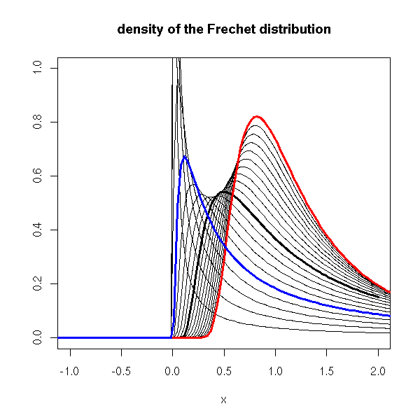
curve(drweibull(x, shape=1), lwd=3, xlim=c(-2,1), ylim=c(0,1),
      ylab="", main="density of the (reverse) Weibull distribution")
for (s in seq(.1,2,by=.1)) {
  curve(drweibull(x, shape=s), add=T)
}
curve(drweibull(x, shape=2), lwd=3, add=T, col='red')
curve(drweibull(x, shape=.5), lwd=3, add=T, col='blue')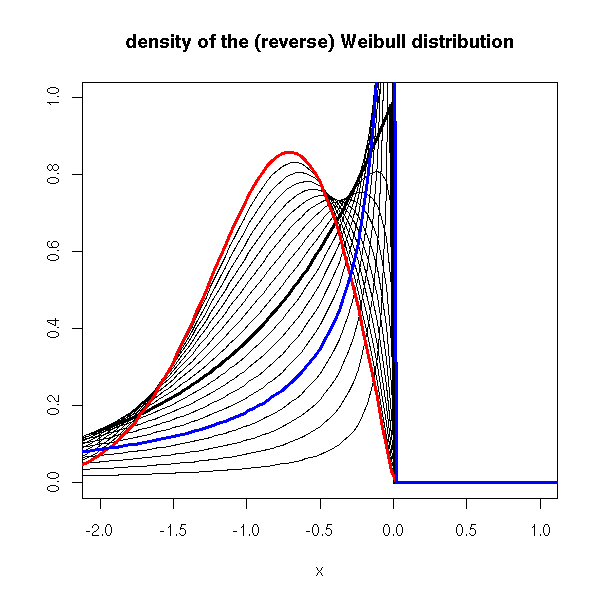
curve(dgumbel(x), lwd=3, xlim=c(-2,2), ylim=c(0,1),
      ylab="", main="density of the Gumbel distribution")
curve(dgev(x, shape=0), lwd=3, xlim=c(-2,2), ylim=c(0,1),
      ylab="", main="density of the GEV distribution")
for (s in seq(-2,2,by=.1)) {
  curve(dgev(x, shape=s), add=T)
}
curve(dgev(x, shape=-1), lwd=3, add=T, col='red')
curve(dgev(x, shape=1), lwd=3, add=T, col='blue')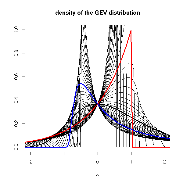
We are now interested in the distribution of X|X>a (i.e., "X given that X>a"), when a becomes large.
TODO: write up this part.

cdf of X, with the "X>a" part in red

x <- read.table("SUNW.csv", header=T, sep=",")
x <- x$Close
x <- diff(log(x))   # Compute the returns
x <- sort(x)
n <- length(x)
m <- floor(.9*n)
y <- (1:n)/n
plot(x,y, type='l', main="empirical cdf of stock returns")
lines(x[m:n], y[m:n], col='red', lwd=3)
cdf of X-a|X>a, same color
plot(x[m:n], y[m:n], col='red', lwd=3,
     type='l', main="empirical conditionnal excess cdf of stock returns")
rescaled cdf of X-a|X>a
plot(x[m:n], (y[m:n] - y[m])/(1-y[m]) , col='red', lwd=3,
     type='l', main="rescaled empirical conditionnal excess cdf of stock returns")
The Generalized Pareto Distribution (GPD) is often a good approximation.
G(x) = 1 - (1 + a/b * x)^ -1/a    if a !=0
G(x) = 1 - exp(-x/b)              if a = 0
Here is its probability distribution function
curve(dgpd(x, shape=0), lwd=3, xlim=c(-.1,2), ylim=c(0,2),
      ylab="", main="density of the Generalized Pereto Distribution (GPD)")
for (s in seq(-2,2,by=.1)) {
  curve(dgpd(x, shape=s), add=T)
}
curve(dgpd(x, shape=-1), lwd=3, add=T, col='red')
curve(dgpd(x, shape=1), lwd=3, add=T, col='blue')
(the more extreme the extreme values, the larger the "shape" parameter -- in our example, we can expect a positive value) and its cdf.
curve(pgpd(x, shape=0), lwd=3, xlim=c(-.1,2), ylim=c(0,1),
      ylab="", main="cdf of the Generalized Pereto Distribution (GPD)")
for (s in seq(-2,2,by=.1)) {
  curve(pgpd(x, shape=s), add=T)
}
curve(pgpd(x, shape=-1), lwd=3, add=T, col='red')
curve(pgpd(x, shape=1), lwd=3, add=T, col='blue')
To estimate this parameter, we can use quantile-quantile plots.
x <- read.table("SUNW.csv", header=T, sep=",")
x <- x$Close
x <- diff(log(x))   # Compute the returns
x <- sort(x)
n <- length(x)
m <- floor(.9*n)
y <- (1:n)/n
op <- par(mfrow=c(3,3), mar=c(2,2,2,2))
for (s in seq(0,2,length=9)) {
  plot(qgpd(ppoints(n-m+1),shape=s), x[m:n],
       xlab='', ylab='')
}
par(op)
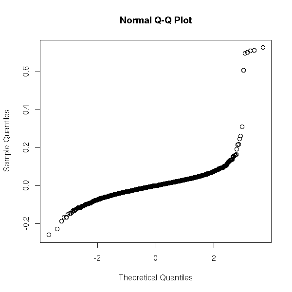
Here, we do not see much: we have the impression that half a dozen points do not follow the same distribution as the others. We could already spot them in the usual quantile-quantile plot.
qqnorm(x)
But there is a slight problem: it might be a good idea to look at X|X>a and try to model its distribution, but how do we choose a in the first place? Where do we truncate the distribution? In other words, where does the tail of the distribution start?
TODO

Sample mean excess plot
(u, e(u))
where e(u) = mean of the (x_i - u), for i such that x_i > u
This could be written:
  mean( (x-u)[x>u] )

x <- sort(x)
e <- rep(NA, length(x))
for (i in seq(along=x)) {
  u <- x[i]
  e[i] <- mean( (x-u)[x>u] )
}
plot(x, e, type='o', main="Sample mean excess plot")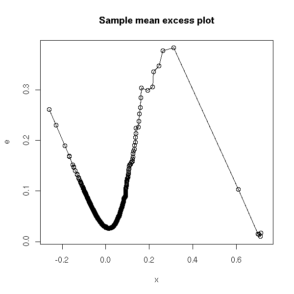
Here is again our pathology. We can see three parts: the part we are not interested in; the "regular" tail, we are interested in; and a few outliers. We choose a at the begining of the regular tail.
(Honestly, I am not really confident about this: there are too many observations in the "irregular tail" to simply forget about them, but too few (and they are too clustered) to be really used.)
TODO: understand...
Let us check another example.
op <- par(mfrow=c(3,3))
for (f in c("SUNW", "ADBE", "ADPT",
            "PCAR", "COST", "INTC",
            "MSFT", "ADCT", "BMET")) {
  x <- read.table(paste(f,".csv", sep=''), header=T, sep=",")
  x <- x$Close
  x <- diff(log(x))   # Compute the returns
  x <- sort(x)
  e <- rep(NA, length(x))
  for (i in seq(along=x)) {
    u <- x[i]
    e[i] <- mean( (x-u)[x>u] )
  }
  plot(x, e, type='o', main="Sample mean excess plot")
}
par(op)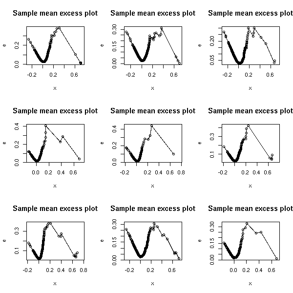
The other tail of those examples.
op <- par(mfrow=c(3,3))
for (f in c("SUNW", "ADBE", "ADPT",
            "PCAR", "COST", "INTC",
            "MSFT", "ADCT", "BMET")) {
  x <- read.table(paste(f,".csv", sep=''), header=T, sep=",")
  x <- x$Close
  x <- -diff(log(x))   # Compute the returns
  x <- sort(x)
  e <- rep(NA, length(x))
  for (i in seq(along=x)) {
    u <- x[i]
    e[i] <- mean( (x-u)[x>u] )
  }
  plot(x, e, type='o', main="Sample mean excess plot")
}
par(op)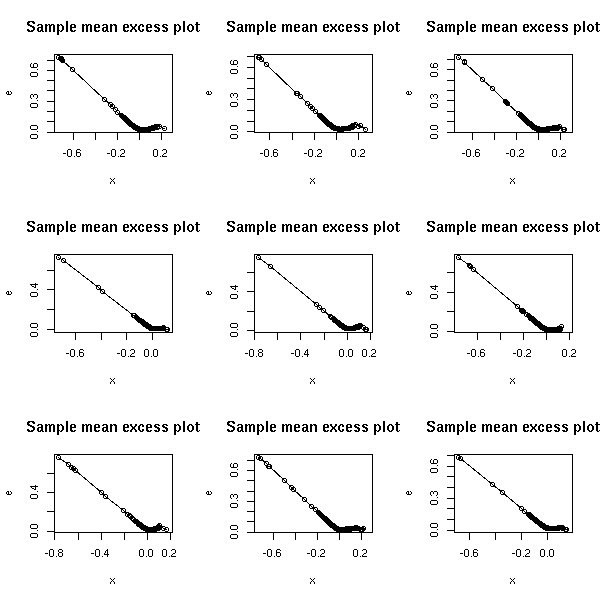
See also
An Application of Extreme Value Theory for Measuring Risk
http://www.unige.ch/ses/metri/gilli/evtrm/evtrm.pdf
http://www.unige.ch/ses/metri/gilli/evtrm/CSDA-08-02-2003.pdf
TODO
Less commonly used distributions are in separate packages. For instance:
evd (extreme value distribution)
gld (generalized lambda distribution)
SuppDists
normalp (generalizations of the gaussian distribution)

This work is licensed under a Creative Commons Attribution-NonCommercial-ShareAlike 2.5 License.
Vincent Zoonekynd
<zoonek@math.jussieu.fr>
latest modification on Sat Jan 6 10:28:20 GMT 2007