
Non-hierarchical clustering (k-means)
Hierarchical Classification (dendogram)
Comparing those two methods
Density estimation
Other packages
We now consider the problem of classifying the observation or the subjects into several groups, several classes. For instance, we have weighted and measured animals and we would like to know if there are several species: do the data form a single cluster or several?
This is called "unsupervised" learning, because we do not know the classes nor even their number. When we know the classes and try to find criteria to assign new observations to a class, we call that "supervised learning" -- it is a regression, with a qualitative variable to predict.
We choose k points, the "centers", and we cluster the data into k classes, assigning each point to its nearest center. We then replace the centers by the center of gravity of the points in their class. And we iterate.
This method has several problems: the result depends on the first centers chosen (we can start again with new centers and compare -- or even adapt the algorithm with genetic algorithms); it is not well-adapted to noisy data; we have to know the number of clusters; the algorithm implicitely assumes that the clusters have the same size (while one application of clustering is "outlier detection", with two classes: one, large, with most of the data, another, smaller, with the outliers); it assigns each point to a class, even if there is some ambiguity (we would like to know if the classification of a new point is ambiguous).
The k-means algorith is very similar.
Explain what the k-means algorithm is.

"the nonhierarchical k means or iterative relocation
algorithm. Each case is initially placed in one of k
clusters, cases are then moved between clusters if it
minimises the differences between cases within a cluster."

x <- rbind(matrix(rnorm(100, sd = 0.3), ncol = 2),
           matrix(rnorm(100, mean = 1, sd = 0.3), ncol = 2))
cl <- kmeans(x, 2, 20)
plot(x, col = cl$cluster, pch=3, lwd=1)
points(cl$centers, col = 1:2, pch = 7, lwd=3)
segments( x[cl$cluster==1,][,1], x[cl$cluster==1,][,2],
          cl$centers[1,1], cl$centers[1,2])
segments( x[cl$cluster==2,][,1], x[cl$cluster==2,][,2],
          cl$centers[2,1], cl$centers[2,2],
          col=2)
Let us try this with my pupils' marks (I spent one year as a high school teacher -- a dreadful experience, that I would not advise to anyone).
# This is not what we want...
load(file="data_notes.Rda") # reads in the "notes" matrix, defined
                            # in a preceding chapter.
cl <- kmeans(notes, 6, 20)
plot(notes, col = cl$cluster, pch=3, lwd=3)
points(cl$centers, col = 1:6, pch=7, lwd=3)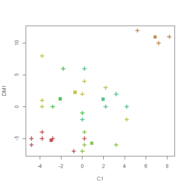
This is not what we want: we got the plot in the first two coordinates of the data set instead of the first two coordinates of the Principal Component Analysis of the data set.
n <- 6
cl <- kmeans(notes, n, 20)
p <- princomp(notes)
u <- p$loadings
x <- (t(u) %*% t(notes))[1:2,]
x <- t(x)
plot(x, col=cl$cluster, pch=3, lwd=3)
c <- (t(u) %*% t(cl$center))[1:2,]
c <- t(c)
points(c, col = 1:n, pch=7, lwd=3)
for (i in 1:n) {
  print(paste("Cluster", i))
  for (j in (1:length(notes[,1]))[cl$cluster==i]) {
    print(paste("Point", j))
    segments( x[j,1], x[j,2], c[i,1], c[i,2], col=i )
  }
}
text( x[,1], x[,2], attr(x, "dimnames")[[1]] )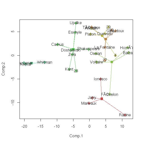
In fact, the "clusplot" already does this. We give it the result of one of the following functions, that are variants of the k-means algorithm.
pam    partitionning around medoids (more robust)
clara  other partitionning, well-suited for large data sets
       (the idea is just to sample from the large data set)
daisy  dissimilarity matrix: qualitative or quantitative variables
dist   dissimilarity matrix: quantitative variables only
fanny  fuzzy clustering
TODO: explain (here or elsewhere, the assumed properties of the clusters for these different methods: same size or not, same shape (variance) or not, etc.)
Here are a few sample results.
library(cluster)
clusplot( notes, pam(notes, 6)$clustering )
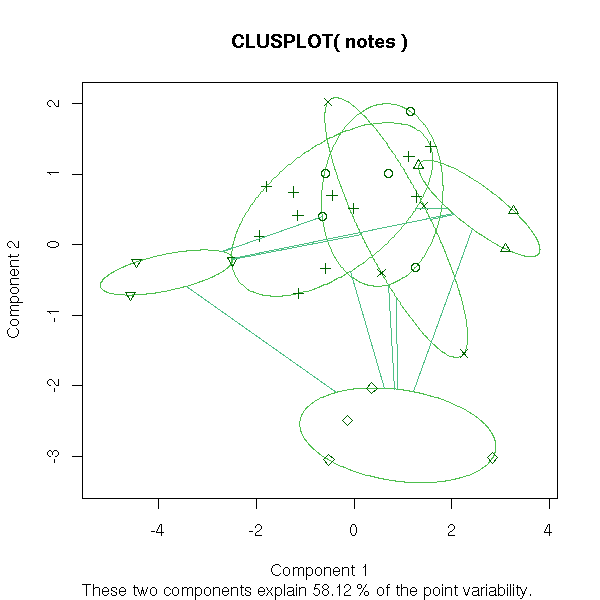
clusplot( notes, pam(notes, 2)$clustering )

clusplot( daisy(notes), pam(notes,2)$clustering, diss=T )
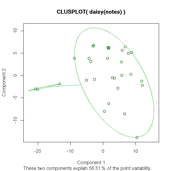
clusplot( daisy(notes), pam(notes,6)$clustering, diss=T )

clusplot(fanny(notes,2))
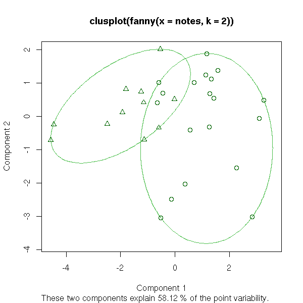
clusplot(fanny(notes,10))

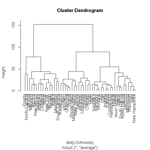
We start with a cloud of n points and we put each point in a class of its own (so we have n classes, each containing a single point). Then, we look for the closest two classes (for a given distance, for instance the distance between their center of gravity -- but other distances will give other results, perhaps more appropriate for some data sets) and we join them into a new class. We now have n-1 classes, all but one containing a single element. Then we iterate. The result can be presented as a dendogram: the leaves are the initial 1-element classes and the various "cuts" (by a horizontal line in the following plot) of the dendogram are various clusterings of the data, into a decreasing number of classes.
data(USArrests)
hc <- hclust(dist(USArrests), "ave")
plot(hc)

plot(hc, hang = -1)
Here is the result with my pupils' marks: I try to plot the tree onto the first two components of the PCA.
plot(hclust(dist(notes)))

p <- princomp(notes)
u <- p$loadings
x <- (t(u) %*% t(notes))[1:2,]
x <- t(x)
plot(x, col="red")
c <- hclust(dist(notes))$merge
y <- NULL
n <- NULL
for (i in (1:(length(notes[,1])-1))) {
  print(paste("Step", i))
  if( c[i,1]>0 ){
    a <- y[ c[i,1], ]
    a.n <- n[ c[i,1] ]
  } else {
    a <- x[ -c[i,1], ]
    a.n <- 1
  }
  if( c[i,2]>0 ){
    b <- y[ c[i,2], ]
    b.n <- n[ c[i,2] ]
  } else {
    b <- x[ -c[i,2], ]
    b.n <- 1
  }
  n <- append(n, a.n+b.n)
  m <- ( a.n * a + b.n * b )/( a.n + b.n )
  y <- rbind(y, m)
  segments( m[1], m[2], a[1], a[2], col="red" )
  segments( m[1], m[2], b[1], b[2], col="red" )
  if( i> length(notes[,1])-1-6 ){
    op=par(ps=30)
    text( m[1], m[2], paste(length(notes[,1])-i), col="red" )
    par(op)
  }
}
text( x[,1], x[,2], attr(x, "dimnames")[[1]] )
Conclusion: either choose the representation as a tree (and forget about PCA, at least for a moment), or only plot the first two or three levels of the tree -- as we did above.
Also see the "mclust" package (Model-based clustering) that models the data as a mixture of gaussians (i.e., as a superposition of clusters).
library(help=mclust)
TODO:
- a tree with no clusters
- a tree with a lot of outliers (i.e., a lot of "horizontal branches")
- a tree with "biological" (balanced) clusters
- a tree with "financial" (unbalanced) clusters

do.it <- function (x, k=3, main="") {
  if (inherits(x, "dist")) {
    d <- x
    x <- sammon(d)$points
  } else {
    d <- dist(x)
    if (!is.vector(x)) {
      x <- sammon(d)$points
    }
  }
  op <- par(mfrow = c(2,2),
            mar = c(3,2,4,2)+.1,
            oma = c(0,0,0,0))
  if (is.vector(x)) {
    hist(x,
         col="light blue",
         xlab="", ylab="", main="Data")
  } else {
    plot(x, main="Data")
  }
  hist(as.vector(d),
       col="light blue",
       xlab="", ylab="", main="Distances")
  plot(hclust(d), labels=FALSE,
       main = "Hierarchical clustering")
  plot(silhouette(cutree(hclust(d),k), d),
       main = "Silhouette")
  par(op)
  mtext(main, line=3, font=2, cex=1.2)
}
do.it(runif(100), k=2,
      main="Random gaussian data")
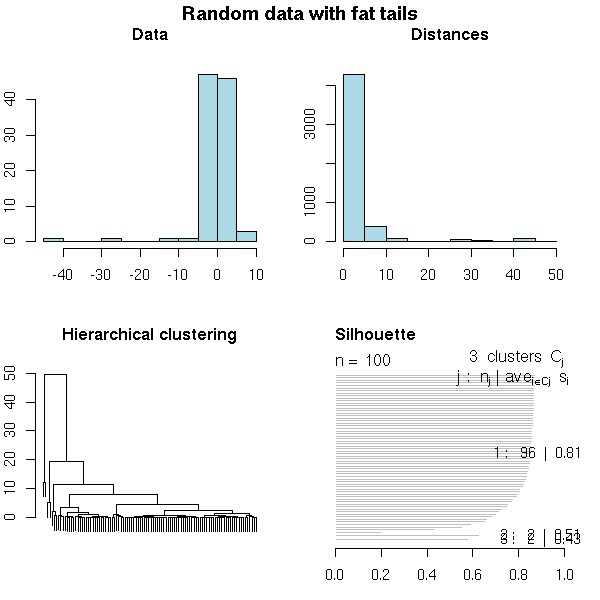
set.seed(1)
x <- rt(100,2)
do.it(x, main="Random data with fat tails")
x <- matrix(rnorm(10000), nr=100, nc=100)
do.it(x, main="High-dimensional random gaussian data")

set.seed(1)
x <- matrix(rt(10000, df=4), nr=100, nc=100)
do.it(x, k=5, main="High-dimensional, fat tails")

N <- 100
x <- rnorm(N, sample(c(-2,2), N, replace=T))
do.it(x, k=2, main="Two real clusters")

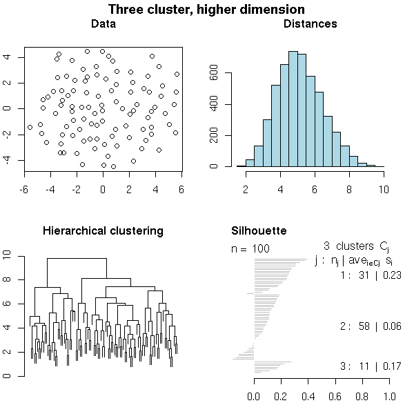
N <- 100  # Number of observations
n <- 10   # Dimension
k <- 3    # Number of clusters
i <- sample( 1:k, N, replace=T )
mu <- matrix(runif(n*k, -2, 2), nr=k, nc=n)
x <- matrix(rnorm(N*n), nc=n) + mu[i,]   # One subject per row
do.it(x, k=3, main="Three cluster, higher dimension")
TODO: Find some financial data
TODO: Find some biological data (multiple alignment)
TODO: Find some bad data (with a lot of horizontal segments)
Hierarchical classification requires you to choose a notion of distance between points and a notion of distance between clusters.
There might be several reasonable choices of a distance between points: for instance, to perform a hierarchical analysis on protein sequences, we can, after aligning them, count the number of differences. We can also weight those differences: if the physico-chemical properties of the amino-acids are similar, the distance will be short, if they are very different, the distance will be higher. (For further analyses, we also have another notion of distance, only available after hierarchical classification: we can measure the distance on the dendogram.)
TODO: give an alignment example
TODO: other distance examples
Cosine distance: scalar product of two (unit) vectors, i.e., the
                 correlation. It is a similarity measure.

TODO: define "similarity measure".

Count data:
  Chi2 : Chi2 of the test for equality.
  Phi2 : ??? This measure is equal to the chi-square measure
             normalized by the square root of the combined frequency.

Binary (or qualitative) data: there are more than a dozen
notions of distance or similarity.
TODO: a reference.
We already mentionned them when dealing with supervised
classification, to assess the quality of the results: we
were comparing the real classes and the predicted classes.
TODO
Consider a cloud of points in the plane. To compute the distance betweem two of those points, one could use the euclidian distance.
N <- 1000
d <- matrix(rnorm(2*N), nc=2)
par(mar=c(2,2,4,2))
plot(d, xlim=c(-2,2), ylim=c(-2,2),
     axes = FALSE,
     xlab="", ylab="",
     main="Contour plot of the Euclidian distance to the origin")
box()
abline(h=0, v=0, lty=3)
x <- seq(min(d[,1]), max(d[,1]), length=100)
y <- seq(min(d[,2]), max(d[,2]), length=100)
z <- outer(x, y, function (x,y) sqrt(x^2 + y^2))
contour(x, y, z,
        add = TRUE,
        col = "blue", lwd = 3)
But if the cloud of points is more elliptical than spherical, this might not be the best choice: in the following plot, points 1 and 2 are at the same euclidian distance from the origin, but point 1 is very far away from the bulk of the cloud.
N <- 5000
library(MASS)
d <- mvrnorm(N, mu=c(0,0), Sigma=matrix(c(1,.8,.8,1),2))
par(mar=c(2,2,4,2))
plot(d, xlim=c(-2,2), ylim=c(-2,2),
     axes = FALSE,
     xlab="", ylab="",
     main="Contour plot of the Euclidian distance to the origin")
box()
abline(h=0, v=0, lty=3)
x <- seq(min(d[,1]), max(d[,1]), length=100)
y <- seq(min(d[,2]), max(d[,2]), length=100)
z <- outer(x, y, function (x,y) sqrt(x^2 + y^2))
contour(x, y, z,
        add = TRUE,
        col = "blue", lwd = 1)
points(sqrt(2)*c(1,-1), sqrt(2)*c(1,1),
       lwd = 10, cex = 5, pch = 4, col = "blue")
text(sqrt(2)*c(1,-1), sqrt(2)*c(1,1) + .1,
     c("2", "1"),
     pos = 3, adj = .5,
     font = 2, cex = 3, col = "blue")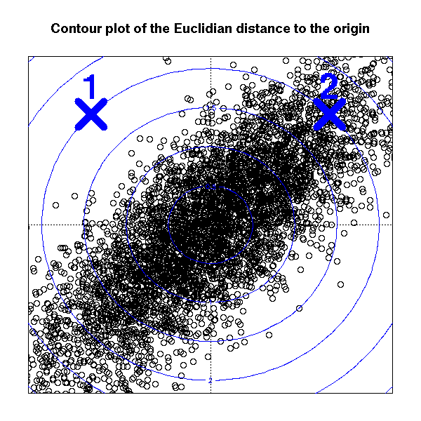
The Mahalanobis distance accounts for this. it is defined as
d(x1, x2) = (x1 - x2)' V^-1 (x1 - x2)
where V is the variance matrix of the cloud of points (either the one corresponding to the gaussian random variable from which the points were samples, if you know it, or an estimation of it).
N <- 1000
V <- matrix(c(1,.8,.8,1),2)
d <- mvrnorm(N, mu=c(0,0), Sigma=V)
par(mar=c(2,2,4,2))
plot(d, xlim=c(-2,2), ylim=c(-2,2),
     axes = FALSE,
     xlab="", ylab="",
     main="Contour plot of the Mahalanobis distance to the origin")
box()
abline(h=0, v=0, lty=3)
x <- seq(min(d[,1]), max(d[,1]), length=100)
y <- seq(min(d[,2]), max(d[,2]), length=100)
z <- outer(x, y, function (x, y) {
  sqrt(apply(rbind(x,y) * solve(V, rbind(x,y)), 2, sum))
} )   # BUG: MEMORY PROBLEM...
contour(x, y, z,
        add = TRUE,
        col = "blue", lwd = 3)
In some situations, some people also advocate the use of the "tracking error distance",
x(x1, x2) = (x1 - x2)' V (x1 - x2)
The rationale could be the following: we think the data is inherently unidimensional and we want to lower the importance of the other, noisy dimensions.
N <- 1000
V <- matrix(c(1,.8,.8,1),2)
d <- mvrnorm(N, mu=c(0,0), Sigma=V)
par(mar=c(2,2,4,2))
plot(d, xlim=c(-2,2), ylim=c(-2,2),
     axes = FALSE,
     xlab="", ylab="",
     main="Contour plot of the Tracking Error distance to the origin")
box()
abline(h=0, v=0, lty=3)
x <- seq(min(d[,1]), max(d[,1]), length=100)
y <- seq(min(d[,2]), max(d[,2]), length=100)
z <- outer(x, y, function (x, y) {
  sqrt(apply(rbind(x,y) * (V %*% rbind(x,y)), 2, sum))
} )
contour(x, y, z,
        add = TRUE,
        col = "blue", lwd = 3)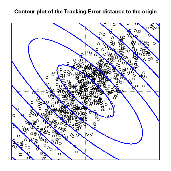
The notion of distance between clusters is slightly trickier. Here are a few examples of such a distance.
d(A,B) = Max { d(a,b) ; a \in A and b \in B }

d(A,B) = Min { d(a,b) ; a \in A and b \in B }

d(A,B) = d(center of gravity of A, center of gravity of B) (actually used?)

d(A,B) = mean of the d(a,b) where a \in A and b \in B    (UPGMA: Unweighted Pair-Groups Method Average)
TODO: plots illustrating those notions.
TODO: Ward's method
Ward's method
Cluster membership is assessed by calculating the total
sum of squared deviations from the mean of a cluster. The
criterion for fusion is that it should produce the
smallest possible increase in the error sum of squares.
Remark: the same data, with different algorithms and/or distances, can produce completely unrelated dendograms.
TODO
Detecting outliers (they form one or several small
clusters, isolated from the rest of the data)

TODO
Non-supervised learning, when you do not know the number
of classes.
The k-means algorithm algorithm and its variants are very fast, well-suited to large data sets, but non-deterministic -- hierarchical clustering is just the opposite.
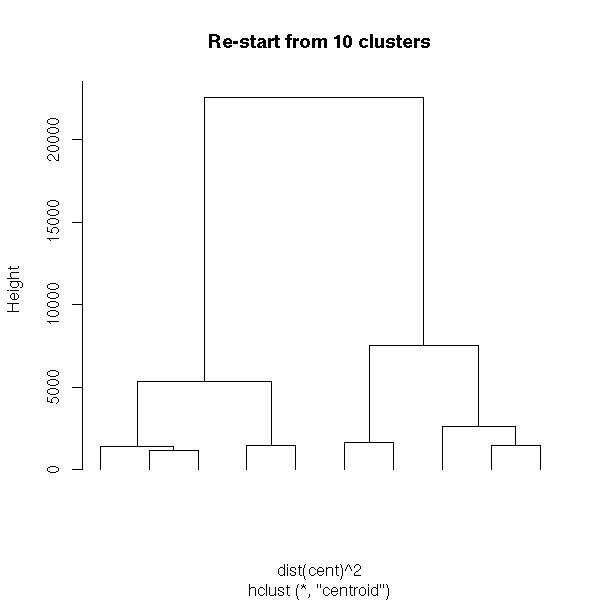
That is why we sometimes mix those two approaches (hybrid clustering): we start with the k-means algorithm to get a few tens or hundreds of classes; then hierarchical clustering on those classes (not on the initial data, too large) to find the number of classes; finally, we can refine, with the k-means algorithm on the newly obtained classes.
TODO Example: do this, following this example (from the manual)
## Do the same with centroid clustering and squared Euclidean distance,
## cut the tree into ten clusters and reconstruct the upper part of the
## tree from the cluster centers.
hc <- hclust(dist(USArrests)^2, "cen")
memb <- cutree(hc, k = 10)
cent <- NULL
for(k in 1:10){
  cent <- rbind(cent, colMeans(USArrests[memb == k, , drop = FALSE]))
}
hc1 <- hclust(dist(cent)^2, method = "cen", members = table(memb))
opar <- par(mfrow = c(1, 2))
plot(hc,  labels = FALSE, hang = -1, main = "Original Tree")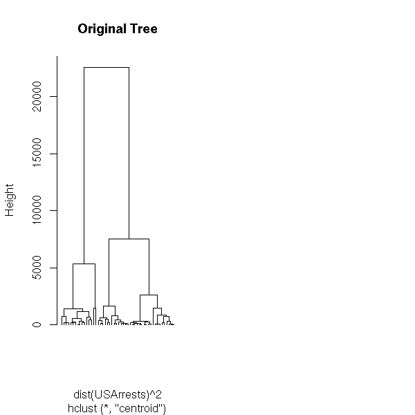
plot(hc1, labels = FALSE, hang = -1, main = "Re-start from 10 clusters")
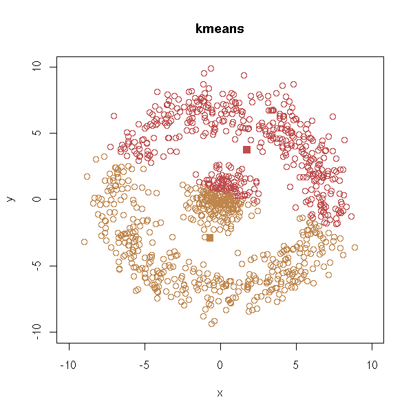
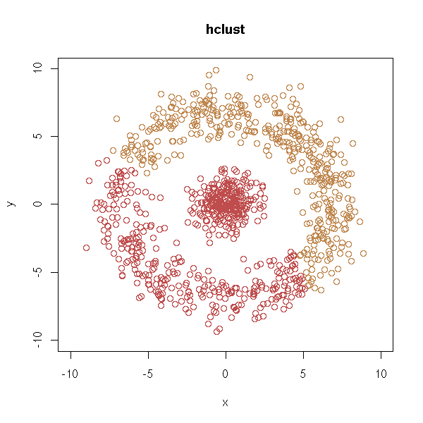
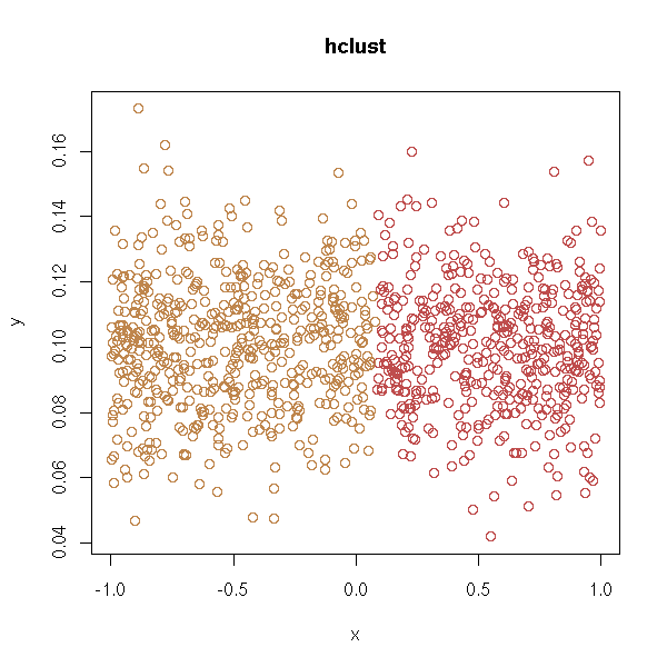
The preceding methods assumed that the clusters were convex, or even spherical. But this is not always the case.
In the following example, we would like the computer to find two clusters...
n <- 1000
x <- runif(n,-1,1)
y <- ifelse(runif(n)>.5,-.1,.1) + .02*rnorm(n)
d <- data.frame(x=x, y=y)
plot(d,type='p', xlim=c(-1,1), ylim=c(-1,1))

With k-means:
test.kmeans <- function (d, ...) {
  cl <- kmeans(d,2)
  plot(d, col=cl$cluster, main="kmeans", ...)
  points(cl$centers, col=1:2, pch=7, lwd=3)
}
test.kmeans(d, xlim=c(-1,1), ylim=c(-1,1))
With hierarchical clustering:
test.hclust <- function (d, ...) {
  hc <- hclust(dist(d))
  remplir <- function (m, i, res=NULL) {
    if(i<0) {
      return( c(res, -i) )
    } else {
      return( c(res, remplir(m, m[i,1], NULL), remplir(m, m[i,2], NULL) ) )
    }
  }
  a <- remplir(hc$merge, hc$merge[n-1,1])
  b <- remplir(hc$merge, hc$merge[n-1,2])
  co <- rep(1,n)
  co[b] <- 2
  plot(d, col=co, main="hclust", ...)
}
test.hclust(d, xlim=c(-1,1), ylim=c(-1,1))
We can also imagine other pathologies, with non-convex clusters.
get.sample <- function (n=1000, p=.7) {
  x1 <- rnorm(n)
  y1 <- rnorm(n)
  r2 <- 7+rnorm(n)
  t2 <- runif(n,0,2*pi)
  x2 <- r2*cos(t2)
  y2 <- r2*sin(t2)
  r <- runif(n)>p
  x <- ifelse(r,x1,x2)
  y <- ifelse(r,y1,y2)
  d <- data.frame(x=x, y=y)
  d
}
d <- get.sample()
plot(d,type='p', xlim=c(-10,10), ylim=c(-10,10))
test.kmeans(d, xlim=c(-10,10), ylim=c(-10,10))
test.hclust(d, xlim=c(-10,10), ylim=c(-10,10))
y <- abs(y)
d <- data.frame(x=x, y=y)
plot(d,type='p', xlim=c(-10,10), ylim=c(0,10))

test.kmeans(d)

test.hclust(d)
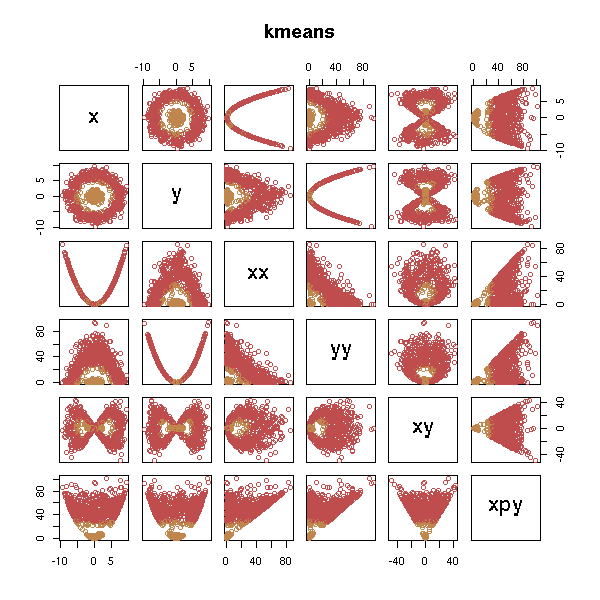
You can try to add variables (this is the same idea that leads to polynomial regression -- or kernel methods).
d <- get.sample()
x <- d$x; y <- d$y
d <- data.frame(x=x, y=y, xx=x*x, yy=y*y, xy=x*y)
test.kmeans(d)

test.hclust(d)

But it does not work, unless we add the "right" variables.
d <- data.frame(x=x, y=y, xx=x*x, yy=y*y, xy=x*y, xpy=x*x+y*y)
test.kmeans(d)
test.hclust(d)

In that kind of situation, if there are only two dimensions, we can try to estimate the corresponding probability density and hope to see two peaks.
help.search("density")
# Suggests:
#   KernSur(GenKern)        Bivariate kernel density estimation
#   bkde2D(KernSmooth)      Compute a 2D Binned Kernel Density Estimate
#   kde2d(MASS)             Two-Dimensional Kernel Density Estimation
#   density(mclust)         Kernel Density Estimation
#   sm.density(sm)          Nonparametric density estimation in 1, 2 or 3 dimensions.
library(KernSmooth)
r <- bkde2D(d, bandwidth=c(.5,.5))
persp(r$fhat)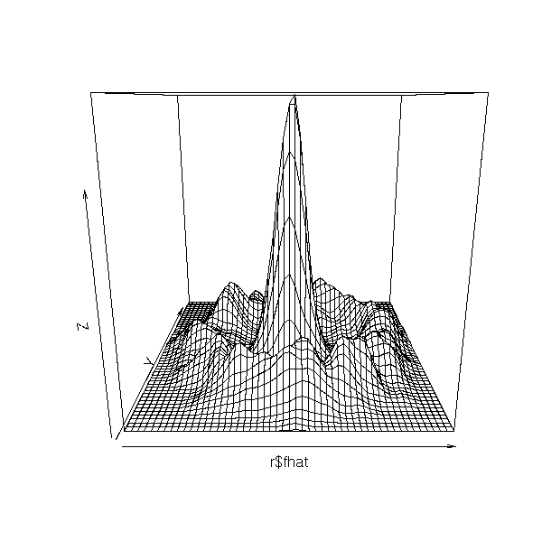
n <- length(r$x1)
plot( matrix(r$x1, nr=n, nc=n, byrow=F),
      matrix(r$x2, nr=n, nc=n, byrow=T),
      col=r$fhat>.001 )
TODO: a similar plot with hexbin?
(We leave it as an exercise to the reader to finish this example, by telling the computer how to find the connected components of the preceding plot and how to use them for forecasting.)
You can use the same idea in a more algorithmitic way as follows: for each observation x, we count the number of observations at a distance at most 0.1 (you can change this value) from x; if there are more than 5 (you can change this value), we say that the observation x is dense, i.e., inside a cluster. We then define an equivalence relation between dense observations by saying that they are in the same cluster if their distance is under 0.1.
http://www.genopole-lille.fr/fr/formation/cib/doc/datamining/DM-Bio.pps
(page 66)
You can implement this idea as follows.
density.classification.plot <- function (x,y,d.lim=.5,n.lim=5) {
  n <- length(x)
  # Distance computation
  a <- matrix(x, nr=n, nc=n, byrow=F) - matrix(x, nr=n, nc=n, byrow=T)
  b <- matrix(y, nr=n, nc=n, byrow=F) - matrix(y, nr=n, nc=n, byrow=T)
  a <- a*a + b*b
  # Which observations are dense (i.e., in a cluster)?
  b <- apply(a<d.lim, 1, sum)>=n.lim
  plot(x, y, col=b)
  points(x,y,pch='.')
}
density.classification.plot(d$x,d$y)
We then have to identify the various clusters.
# Beware: the following code is very recursive -- but, by default,
# R limits the size of the function calls stack to 500 elements.
# We first increment this value.
options(expressions=10000)

density.classification.plot <- function (x,y,d.lim=.5,n.lim=5) {
  n <- length(x)
  # Distance computations
  a <- matrix(x, nr=n, nc=n, byrow=F) - matrix(x, nr=n, nc=n, byrow=T)
  b <- matrix(y, nr=n, nc=n, byrow=F) - matrix(y, nr=n, nc=n, byrow=T)
  a <- a*a + b*b
  # Which observations are dense (in a cluster)?
  b <- apply(a<d.lim, 1, sum)>=n.lim
  # We sort the observations
  cl <- rep(0,n)
  m <- 1
  numerote <- function (i,co,cl) {
    print(paste(co, i))
    for (j in (1:n)[ a[i,]<d.lim & b & cl==0 ]) {
      #print(paste("  ",j))
      cl[j] <- co
      try( cl <- numerote(j,co,cl) )   # Too recursive...
    }
    cl
  }
  for (i in 1:n) {
    if (b[i]) { # Are we in a cluster?
      # Cluster number
      if (cl[i] == 0) {
        co <- m
        cl[i] <- co
        m <- m+1
      } else {
        co <- cl[i]
      }
      # We number the nearby points
      #print(co)
      cl <- numerote(i,co,cl)
    }
  }
  plot(x, y, col=cl)
  points(x,y,pch='.')
}
density.classification.plot(d$x,d$y)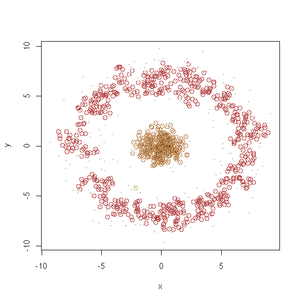
Let us try again, in a more iterative way.
density.classification.plot <- function (x,y,d.lim=.5,n.lim=5, ...) {
  n <- length(x)
  # Distance computation
  a <- matrix(x, nr=n, nc=n, byrow=F) - matrix(x, nr=n, nc=n, byrow=T)
  b <- matrix(y, nr=n, nc=n, byrow=F) - matrix(y, nr=n, nc=n, byrow=T)
  a <- a*a + b*b
  # Which observations are dense (in a cluster)?
  b <- apply(a<d.lim, 1, sum)>=n.lim
  # We sort the observations
  cl <- rep(0,n)
  m <- 0
  for (i in 1:n) {
    if (b[i]) { # Are we in a cluster?
      # Cluster number
      if (cl[i] == 0) {
        m <- m+1
        co <- m
        cl[i] <- co
        print(paste("Processing cluster", co))
        done <- F
        while (!done) {
          done <- T
          for (j in (1:n)[cl==co]) {
            l <- (1:n)[ a[j,]<d.lim & b & cl==0 ]
            if( length(l)>0 ) {
              done <- F
              for (k in l) {
                cl[k] <- co
                #print(k)
              }
            }
          }

        }
      } else {
        # Already processed cluster: pass
      }
    }
  }
  plot(x, y, col=cl, ...)
  points(x,y,pch='.')
}
density.classification.plot(d$x,d$y)
Let us play with the parameters.
op <- par(mfrow=c(3,3))
for (d.lim in c(.2,1,2)) {
  for (n.lim in c(3,5,10)) {
    density.classification.plot(d$x,d$y,d.lim,n.lim,
      main=paste("d.lim = ",d.lim, ",  n.lim = ",n.lim, sep=''))
  }
}
par(op)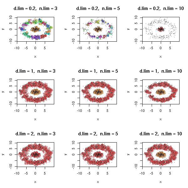
amap:  parallelized hclust, robust PCA
party: mob (model-based recursive partitionning)
       cforest (random forest ensemble algorithm on
       conditional inference trees)
cba

This work is licensed under a Creative Commons Attribution-NonCommercial-ShareAlike 2.5 License.
Vincent Zoonekynd
<zoonek@math.jussieu.fr>
latest modification on Sat Jan 6 10:28:19 GMT 2007