Principal Component Analysis (PCA)
Distance-based methods
SOM (Self-Organizing Maps)
Simple Correspondance Analysis (CA)
Multiple Correspondance Analysis
Log-linear model (Poisson Regression)
Discriminant Analysis
Canonical analysis
Kernel methods
Neural networks
Dimension reduction: TODO: Rewrite/Remove this section
TODO: to sort
There are two kind of methods in multidimensional statistics: Factorial Methods, in which we project the data on a vector space, trying to lose as little information as possible; and Classification Methods, that try to cluster the points.
There are three main techniques among the Factorial Methods: Principal Component Analysis (PCA, with several quantitative variables), Correspondance Analysis (CA, two quanlitative variables, represented by a contingency table) and Multiple Correspondance Analysis (MCA, more that two variables, all quantitative).
The following table summarizes this:
Method    Quantitative variables    Qualitative variables
----------------------------------------------------------
PCA       several                   none
MDS       several                   none
CA        none                      two
MCA       none                      several
There are other, non symetric, methods: one variable plays a special role, is given a different emphasis than the others (usually, we try to predict or explain one variable from the others).
Method                 Quantitative v.    Qualitative v.    Variable to predict
----------------------------------------------------------------------------------
regression             several          several             quantitative
anova                  none             one                 quantitative
logistic regression    several          several             binary
Poisson regression     several          several             counting
logistic regression    several          several             ordered (qualitative)
discriminant analysis  several          one
CART                   several          several             binary
...
Here is a first presentation of PCA. We have a cloud of points in a high-dimensional space, too large for us to see something in it. The PCA will give us a subspace of reasonable dimension so that the projection onto this subspace retains "as much information as possible", i.e., so that the so that the projected cloud of points be as "dispersed" as possible. In other words, it reduces the dimension of the cloud of points, it helps choose a point of view to look at the cloud of points.
The algorithm is the following. We first translate the data so that its center of gravity be at the origin (always a good thing when you plan to use linear algebra). Then, we try to rotate it so that the standard deviation of the first coordinate be as large as possible (and then the second, third, etc.): this is equivalent to diagonalizing the variance-covariance matrix (it is a (positive) real symetric matrix, hence it is diagonalizable in an orthonormal basis), starting with the eigen vectors of largest eigen value. The first axis of this new coordinate system corresponds to an approximation of the cloud of points by a 1-dimensional space; if you want an approximation by a k-dimensional subspace, just take the first k eigen vectors.
To choose the dimension of that subspace, we can look (graphically) at the eigen values and we stop when they start dropping (if they decrease slowly, we are in a bad situation: with our linear goggles, the data is inherently high-dimensional).
One may also see PCA as an analogue of the least squares method to find a line that goes as "near" the points as possible -- to simplify, let us assume there are just two dimensions. But while the least squares method is asymetric (the two variables play different roles: they are not interchangeable, we try to predict one from the others, we measure the distance parallel to one coordinate axis), the PCA is symetric (the distance is measured orthogonally to the line we are looking for).
Here is yet another way of presenting PCA. We model the data as X = Y + E, where X is the noisy data we have (in an n-dimensional space), Y is the real data (without the noise), in a smaller, k-dimensional space, and E is an error term (the noise). We want to find the k-dimensional space where Y lives.
You can also see PCA as a game on a table of numbers (it is not as childish as it seems: it is actually a description of correspondance analysis). Thus, we can switch the role of rows and columns: on the one hand, we try to find similarities or differences between subjects, on the other, similarities or differences between variables. (There are two matrices to diagonalize, A*t(A) and t(A)*A, but but it suffices to diagonalize one: they have the same non-zero eigen values and the eigen vectors of one can easily be obtained from those of the other.) We usually ask that the variables be centered (and, often, normalized). We can plot both the variables on the same graph as the subjects: the variables will lie on the unit sphere; thei projection on the subspace spanned by the first two eigen vectors is the "correlation circle".
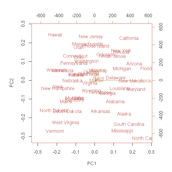
After performing the PCA, we can add new subjects on the plot (test (out-of-sample) subjects; fictitious sujbects, representative of certain classes of subjects): just use the "predict" function. Dually, we can add variables (for explanatory reasons), Of those variables are qualitative, we actually add an "average subject" for each value of this variable. This is often called a "biplot", because both subjects (in black) and variables (in red) appear on the plot.
data(USArrests)
p <- prcomp(USArrests)
biplot(p)
TODO: find a situation where you really want to add
variables and/or subjects.

n <- 100   # Number of subjects
nn <- 10   # Number of out-of-sample subjects
k <- 5     # Number of variable
kk <- 3    # Number of new variables
x <- matrix(rnorm(n*k),  nr=n,  nc=k)
x <- t(rnorm(k) + t(x))                   # Initial data
y <- matrix(rnorm(n*kk), nr=n,  nc=kk)    # New variables
z <- matrix(rnorm(nn*k), nr=nn, nc=k)     # New subjects

r <- prcomp(x)
# I check that my change-of-base formulas were right
all(abs(    t(r$center + t(x %*% r$rotation))  -  r$x    )<1e-8)
# Subjects coordinates
t(r$center + t(x %*% r$rotation))
# Out-of-sample subject coordinates
t(r$center + t(z %*% r$rotation))
# For each new variable, we add an "average" subject
# (more precisely: x %*% t(yy[1,]) = orthogonal projection of
# y[,1] on the subspace spanned by the columns of x).
yy <- t(lm(y~x-1)$coef)
t(r$center + t(yy %*% r$rotation))
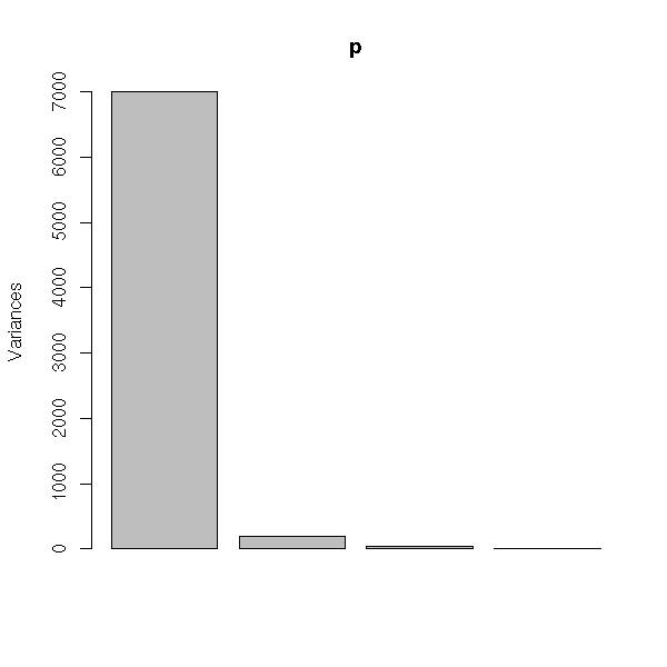
Here are the eigen values. They are plummeting: this means that the PCA is meaningful and that we can retain only the eigen vectors with the highest eigenvalues (here, the first: we could have done a 1-dimensional plot (a histogram)).
plot(p)
There is also a "prcomp" functions, that does the same computations, with a few more limitations (namely, you should have more observations that variables): do not use it.
The vocabulary used with principal components analysis may surprise you: people speak of "loadings" where you would expect "rotation matrix" and "scores" where you think "new coordinates".
In the preceeding plot, the old basis vectors are in red. There is the correlation circle -- those vectors lie on the unit sphere, which we project on the first two eigen vectors (it should not be called a circle but a disc -- the projection of a sphere is a disc, not a circle).
a <- seq(0,2*pi,length=100)
plot( cos(a), sin(a),
      type = 'l', lty = 3,
      xlab = 'comp 1', ylab = 'comp 2',
      main = "Correlation circle")
v <- t(p$rotation)[1:2,]
arrows(0,0, v[1,], v[2,], col='red')
text(v[1,], v[2,],colnames(v))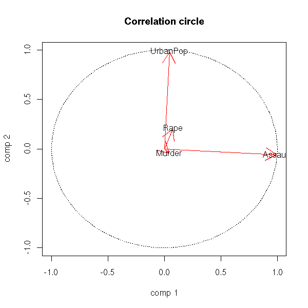
Here is a situation where PCA is not relevant (my pupils's marks, when I was a high school teacher).
# Copy-pasted with the help of the "deparse" command:
# cat( deparse(x), file='foobar')
notes <- matrix( c(15, NA, 7, 15, 11, 7, 7, 8, 11, 11, 13,
6, 14, 19, 9, 8, 6, NA, 7, 14, 11, 13, 16, 10, 18, 7, 7,
NA, 11, NA, NA, 6, 15, 5, 11, 7, 3, NA, 3, 1, 10, 1, 1,
18, 13, 2, 2, 0, 7, 9, 13, NA, 19, 0, 17, 8, 2, 9, 2, 5,
12, 0, 8, 12, 8, 4, 8, 0, 5, 5.5, 1, 12, 4, 13, 5, 11, 6,
0, 7, 8, 11, 9, 9, 9, 14, 8, 5, 8, 5, 5, 12, 6, 16.5,
13.5, 15, 3, 10.5, 1.5, 10.5, 9, 15, 7.5, 12, 13.5, 4.5,
13.5, 13.5, 6, 12, 7.5, 9, 6, 13.5, 13.5, 15, 13.5, 6, NA,
13.5, 4.5, 14, NA, 14, 14, 14, 8, 16, NA, 6, 6, 12, NA, 7,
15, 13, 17, 18, 5, 14, 17, 17, 13, NA, NA, 16, 14, 18, 13,
17, 17, 8, 4, 16, 16, 16, 10, 15, 8, 10, 13, 12, 14, 8,
19, 7, 7, 9, 8, 15, 16, 8, 7, 12, 5, 11, 17, 13, 13, 7,
12, 15, 8, 17, 16, 16, 6, 7, 11, 15, 15, 19, 12, 15, 16,
13, 19, 14, 4, 13, 13, 19, 11, 15, 7, 20, 16, 10, 12, 16,
14, 0, 0, 11, 9, 4, 10, 0, 0, 5, 11, 12, 7, 12, 17, NA, 6,
6, 9, 7, 0, 7, NA, 15, 3, 20, 11, 10, 13, 0, 0, 6, 1, 5,
6, 5, 4, 2, 0, 8, 9, NA, 0, 11, 11, 0, 7, 0, NA, NA, 7, 0,
NA, NA, 6, 9, 6, 4, 5, 4, 3 ), nrow=30)
notes <- data.frame(notes)
# These are not the real names
row.names(notes) <-
c("Anouilh", "Balzac", "Camus", "Dostoievski",
"Eschyle", "Fenelon", "Giraudoux", "Homer",
"Ionesco", "Jarry", "Kant", "La Fontaine", "Marivaux",
"Nerval", "Ossian", "Platon", "Quevedo", "Racine",
"Shakespeare", "Terence", "Updike", "Voltaire",
"Whitman", "X", "Yourcenar", "Zola", "27", "28", "29",
"30")
attr(notes, "names") <- c("C1", "DM1", "C2", "DS1", "DM2",
"C3", "DM3", "DM4", "DS2")
notes <- as.matrix(notes)
notes <- t(t(notes) - apply(notes, 2, mean, na.rm=T))
# Get rid of NAs
notes[ is.na(notes) ] <- 0
# plots
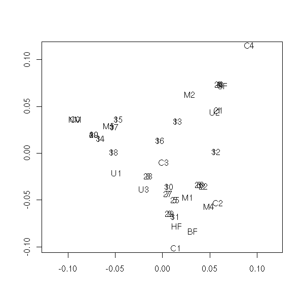
plot(princomp(notes))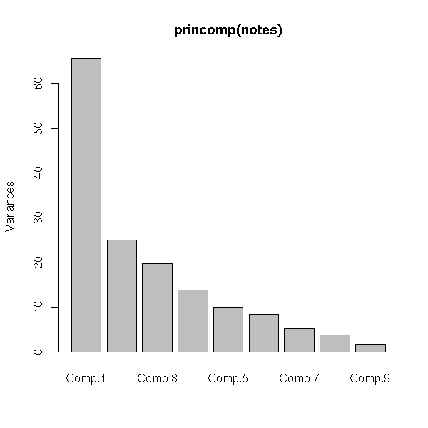
biplot(princomp(notes))
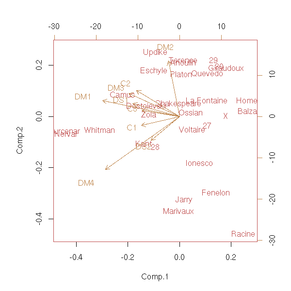
Here, we gave the same weight to each mark and each subject; we could have give more weight to some marks, to reflect their nature (test or homework) or the weight of the subjects for the final exam (e.g., A-level): it is the same algorithm, only the scalar product on the space changes.
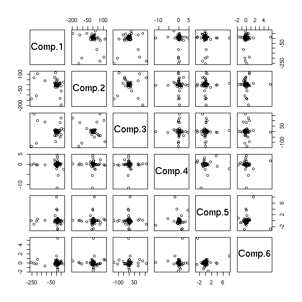
The "biplot" command anly gives the first two dimensions: we can sometimes see more with the "pairs" command.
pairs(princomp(notes)$scores, gap=0)
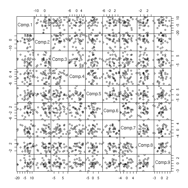
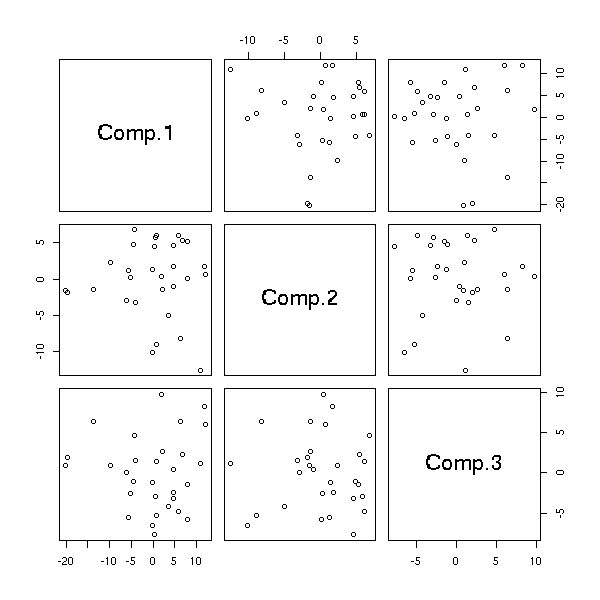
pairs(princomp(notes)$scores[,1:3])
p <- princomp(notes)
pairs( rbind(p$scores, p$loadings)[,1:3],
       col=c(rep(1,p$n.obs),rep(2, length(p$center))),
       pch=c(rep(1,p$n.obs),rep(3, length(p$center))),
     )
We leave it to the reader to add red arrows (instead of red points) for the variables -- actually, the "pairs" function is not very configurable: the different panels take as arguments the coordinates of the points to draw, while one could want to plot, in the same panel, very different things -- but we do not even have the row and column numbers... The corresponding function in the "lattice" library seems scarcely more configurable.
library(lattice)
splom(as.data.frame(
  princomp(notes)$scores[,1:3]
))

Here is another situation where one could want to use PCA: the classification of texts in a corpus. The rows of the table (the subjects) are the texts, the columns are the words (the vocabulary), the values are the number of occurrences of the words in the text. As the dimension of the space (the number of columns) is rather high (several thousands), it is not very easy to compute the covariance matrix, let alone diagonalize it. Yet, one can perform the PCA, in an approximate way, with neural networks.
http://www.loria.fr/projets/TALN/actes/TALN/articles/TALN02.pdf
Here is another means of tackling the same problem, without PCA but still with geometry in high-dimensional spaces:
http://www.perl.com/lpt/a/2003/02/19/engine.html
To understand what PCA really is, how it works, let us implement it ourselves. Here is one possible implementation.
my.acp <- function (x) {
  n <- dim(x)[1]
  p <- dim(x)[2]
  # Translation, to use linear algebra
  centre <- apply(x, 2, mean)
  x <- x - matrix(centre, nr=n, nc=p, byrow=T)
  # diagonalizations, base changes
  e1 <- eigen( t(x) %*% x, symmetric=T )
  e2 <- eigen( x %*% t(x), symmetric=T )
  variables <- t(e2$vectors) %*% x
  subjects <- t(e1$vectors) %*% t(x)
  # The vectors we want are the columns of the
  # above matrices. To draw them, with the "pairs"
  # function, we have to transpose them.
  variables <- t(variables)
  subjects <- t(subjects)
  eigen.values <- e1$values
  # Plot
  plot( subjects[,1:2],
        xlim=c( min(c(subjects[,1],-subjects[,1])),
                max(c(subjects[,1],-subjects[,1])) ),
        ylim=c( min(c(subjects[,2],-subjects[,2])),
                max(c(subjects[,2],-subjects[,2])) ),
        xlab='', ylab='', frame.plot=F )
  par(new=T)
  plot( variables[,1:2], col='red',
        xlim=c( min(c(variables[,1],-variables[,1])),
                max(c(variables[,1],-variables[,1])) ),
        ylim=c( min(c(variables[,2],-variables[,2])),
                max(c(variables[,2],-variables[,2])) ),
        axes=F, xlab='', ylab='', pch='.')
  axis(3, col='red')
  axis(4, col='red')
  arrows(0,0,variables[,1],variables[,2],col='red')
  # Return the data
  invisible(list(data=x, centre=centre, subjects=subjects,
                 variables=variables, eigen.values=eigen.values))
}

n <- 20
p <- 5
x <- matrix( rnorm(p*n), nr=n, nc=p )
my.acp(x)
title(main="ACP by hand")
To check we did not make any error in implementing the algorithm, we can compare the result with that of the "printcomp" command.
biplot(princomp(x))
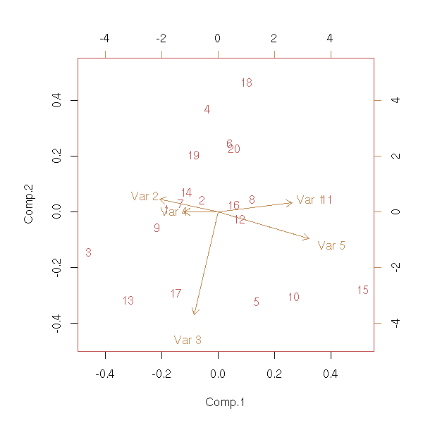
Exercise: Add the subject names; the variable names; plot the first three dimensions of the PCA (not just the first two), as with the "pairs" command; add new variables to the plot (if it is a quantitative variable, apply the same base change, if it is a qualitative variable, compute an average subject for each value of this variable and perform the base change).
Exercice: Modify the preceding code by replacing the "eigen" function by the "svd" command, that performs a Singular Value Decomposition.
TODO
There are several kind of PCA: centered or not, normalized (based on the correlations matrix) or not (based on the variance-covariance matrix).
prcomp(x, center=TRUE, scale.=FALSE) # default
Let us first consider the centered non-normalized principal component analysis, i.e., that based on the variance-covariance matrix.
TODO: This was written for the "princomp" function, not the "prcomp" one -- actually, the problems disappear.
d <- USArrests[,1:3]             # Data
dd <- t(t(d)-apply(d, 2, mean))  # Centered data
m <- cov(d)                      # Covariances matrix
e <- eigen(m)                    # Eigen values and eigen vectors
p <- princomp( ~ Murder + Assault + UrbanPop, data = USArrests)
The change-of-base matrix is the same in both cases:
> e$vectors
            [,1]        [,2]        [,3]
[1,] -0.04181042 -0.04791741  0.99797586
[2,] -0.99806069 -0.04410079 -0.04393145
[3,] -0.04611661  0.99787727  0.04598061

> unclass(p$loadings)
              Comp.1      Comp.2      Comp.3
Murder   -0.04181042 -0.04791741  0.99797586
Assault  -0.99806069 -0.04410079 -0.04393145
UrbanPop -0.04611661  0.99787727  0.04598061
and so are the coordinates:
> p$scores[1:3,]
            Comp.1     Comp.2    Comp.3
Alabama  -64.99204 -10.660459  2.188264
Alaska   -91.34472 -21.676617 -2.651214
Arizona -123.68089   8.979374 -4.437864

> (dd %*% p$loadings) [1:3,]
            Comp.1     Comp.2    Comp.3
Alabama  -64.99204 -10.660459  2.188264
Alaska   -91.34472 -21.676617 -2.651214
Arizona -123.68089   8.979374 -4.437864
Let us now look at the normalized principal component analysis: we do not simply center each column of the matrix, we normalize them.
d <- USArrests[,1:3]
dd <- apply(d, 2, function (x) { (x-mean(x))/sd(x) })
The variance-covariance matrix of this new matrix is the correlation matrix of the initial matrix.
> cov(dd)
             Murder   Assault   UrbanPop
Murder   1.00000000 0.8018733 0.06957262
Assault  0.80187331 1.0000000 0.25887170
UrbanPop 0.06957262 0.2588717 1.00000000

> cor(d)
             Murder   Assault   UrbanPop
Murder   1.00000000 0.8018733 0.06957262
Assault  0.80187331 1.0000000 0.25887170
UrbanPop 0.06957262 0.2588717 1.00000000
Let us go on with the computations:
m <- cov(dd)
e <- eigen(m)
p <- princomp( ~ Murder + Assault + UrbanPop, data = USArrests, cor=T)
We got the right change-of-base matrix:
> e$vectors
          [,1]        [,2]       [,3]
[1,] 0.6672955  0.30345520  0.6801703
[2,] 0.6970818  0.06713997 -0.7138411
[3,] 0.2622854 -0.95047734  0.1667309

> unclass(p$loadings)
            Comp.1      Comp.2     Comp.3
Murder   0.6672955 -0.30345520  0.6801703
Assault  0.6970818 -0.06713997 -0.7138411
UrbanPop 0.2622854  0.95047734  0.1667309
But the coordinates are not the same...
> p$scores[1:3,]
             Comp.1     Comp.2     Comp.3
  Alabama 1.2508055 -0.9341207  0.2015063
  Alaska  0.8006592 -1.3941923 -0.6532667
  Arizona 1.3542765  0.8368948 -0.8488785

> (dd %*% e$vectors) [1:3,]
               [,1]       [,2]       [,3]
  Alabama 1.2382343  0.9247323  0.1994810
  Alaska  0.7926121  1.3801799 -0.6467010
  Arizona 1.3406654 -0.8284836 -0.8403468
However, the error is always the same (up to the sign, which is meaningless):
>  p$scores[1:3,] /  (dd %*% e$vectors) [1:3,]
            Comp.1    Comp.2   Comp.3
  Alabama 1.010153 -1.010153 1.010153
  Alaska  1.010153 -1.010153 1.010153
  Arizona 1.010153 -1.010153 1.010153
The difference comes from the fact that there are two definitions of covariance, one in which you divide ny n, another in which you divide by n-1.
> dim(d)
[1] 50  3
> sqrt(50/49)
[1] 1.010153
TODO: this is not the right place.
Later, with LDA.

for i in `ls *.txt | cat_rand | head -20`
do
  perl -n -e 'BEGIN {
                foreach ("a".."z") { $a{$_}=0 }
              };
              y/A-Z/a-z/;
              s/[^a-z]//g;
              foreach (split("")) { $a{$_}++ }
              END {
                foreach("a".."z"){print "$a{$_} "}
              }' <$i
  echo E
done > ling.txt
# Then the same thing in a directory containing French texts

b <- read.table('ling.txt')
names(b) <- c(letters[1:26], 'language')
a <- b[,1:26]
a <- a/apply(a,1,sum)
biplot(princomp(a))
plot(hclust(dist(a)))

kmeans.plot <- function (data, n=2, iter.max=10) {
  k <- kmeans(data,n,iter.max)
  p <- princomp(data)
  u <- p$loadings
  # The observations
  x <- (t(u) %*% t(data))[1:2,]
  x <- t(x)
  # The centers
  plot(x, col=k$cluster, pch=3, lwd=3)
  c <- (t(u) %*% t(k$center))[1:2,]
  c <- t(c)
  points(c, col = 1:n, pch=7, lwd=3)
  # A segment joining each observation to its group center
  for (i in 1:n) {
    for (j in (1:length(data[,1]))[k$cluster==i]) {
      segments( x[j,1], x[j,2], c[i,1], c[i,2], col=i )
    }
  }
  text( x[,1], x[,2], attr(x, "dimnames")[[1]] )
}
kmeans.plot(a,2)
# plot(lda(a,b[,27])) # Bug?
# plot(lda(as.matrix(a),b[,27])) # Newer bug?
Actually, computers do not perform Principal Component Analysis as we have just seen, by computing the variance-covariance matrix and diagonalizing it.
TODO
Principal component analysis assumes that the data is gaussian. If it is not, we can replace the values by their rank. But then, the variables follow a uniform distribution; We can transform those uniform data to get a gaussian distribution.
n <- 100
v <- .1
a <- rcauchy(n)
b <- rcauchy(n)
c <- rcauchy(n)
d <- data.frame( x1 =  a+b+c+v*rcauchy(n),
                 x2 =  a+b-c+v*rcauchy(n),
                 x3 =  a-b+c+v*rcauchy(n),
                 x4 = -a+b+c+v*rcauchy(n),
                 x5 =  a-b-c+v*rcauchy(n),
                 x6 = -a+b-c+v*rcauchy(n) )
biplot(princomp(d))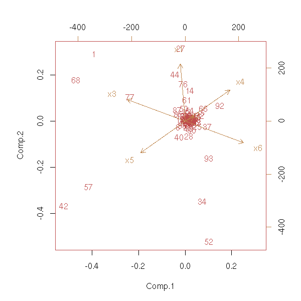
rank.and.normalize.vector <- function (x) {
  x <- (rank(x)-.5)/length(x)
  x <- qnorm(x)
}
rank.and.normalize <- function (x) {
  if( is.vector(x) )
    return( rank.and.normalize.vector(x) )
  if( is.data.frame(x) ) {
    d <- NULL
    for (v in x) {
      if( is.null(d) )
        d <- data.frame( rank.and.normalize(v) )
      else
        d <- data.frame(d, rank.and.normalize(v))
    }
    names(d) <- names(x)
    return(d)
  }
  stop("Data type not handled")
}
biplot(princomp(apply(d,2,rank.and.normalize)))
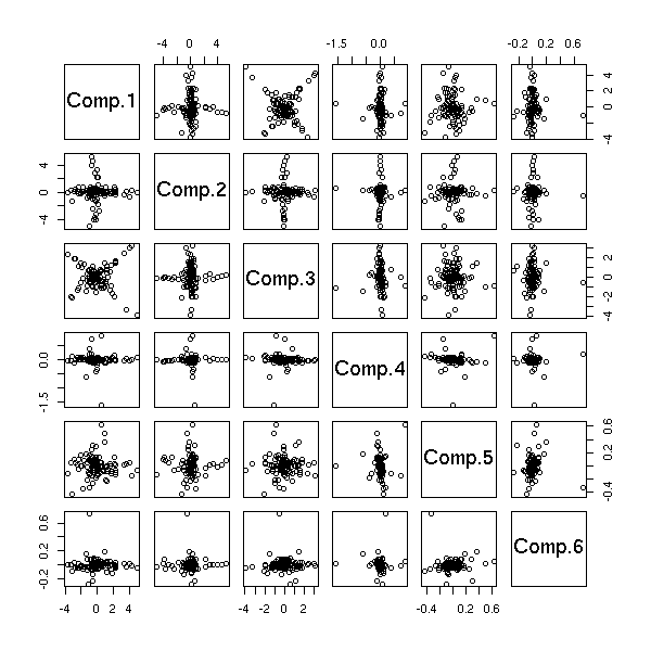
Let us check on the other components of the PCA.
pairs( princomp(d)$scores )
pairs( princomp(apply(d,2,rank.and.normalize))$scores )
For non-linear problems, we can first embed our space in a larger one, with an application such as
(x,y) |--> (x^2, x*y, y^2).
In fact, as the PCA only involves scalar products, we do not really need to compute those new coordinates: it suffices to replace all the occurrences of the scalar product <x,y> by that of the new space (this function, that expresses the scalar product in the new space from the coordinates in the old space, is called a kernel -- and you can take any kernel).
TODO: an example
We shall reuse that idea later (to use a kernel to dive into a higher-dimensional space to linearize a non-linear problem) when we speak of SVM (Support Vector Machines).
http://www.kernel-machines.org/papers/talk-dagm99_4.ps.gz
TODO:
library(kernlab)
?kpca
Principal Component Analysis tries to find a plane (more generally, a subspace of reasonable dimension) in which (the orthogonal projection of) the data is as dispersed as possible, the dispersion being measured with the variance matrix.
Projection pursuit is a generalization of PCA in which one looks for a subspace which maximizes some "interestingness" criterion -- and everyone can define their own criterion. For instance, it could be a measure of the dispersion of the data (based on the variance matrix or on more robust dispersion estimators) or a measure of the non-gaussianity of the data (kurtosis, skewness, etc.).
Those measures of interestingness are called "indices".
The most common Projection Pursuits are PCA, ICA (Independant Component Analysis)m and robust PCA (replace the 1-dimensional variance you are trying to maximize by a robust equivalent).
http://www.r-project.org/useR-2006/Slides/Fritz.pdf
library(pcaPP)
There is also a function called "ppr" (projection pursuit regression) but it seems to do something competely different: variable selection for linear regression, with several variables to predict.
TODO: Give an example
TODO
The grand tour is an animation, a continuous family of projections of the cloud of points onto a 2-dimensional space, obtained by interpolation between random projections: you are supposed to look at it until you see something (clusters, artefacts, alignments, etc.).
GGobi can display grand tours.
http://www.ggobi.org/
The guided tour is a variant of the grand tour, where one interpolates between local maxima of a projection pursuit function instead of random projections.
http://citeseer.ist.psu.edu/cook95grand.html
At first sight, it looks very similar to Principal component analysis -- but it is very different. The general idea is that the variables we are looking at are linear combinations of independant random variables; and we want to recover those random variables. The only assumption is that the random variables we are looking for are independant (well, actually, there is another assumption: those random variables have to be non-gaussian).
ICA has been mainly used in signal processing, the initial example being the cocktail party problem: you have two microphones (or two ears) and you are hearing two conversations at the same time; you want to separate them. Similarly, ICA has also been used to analyze EEG (electroencephalograms).
TODO: 2-dimensional applications, image compression, feature extraction.
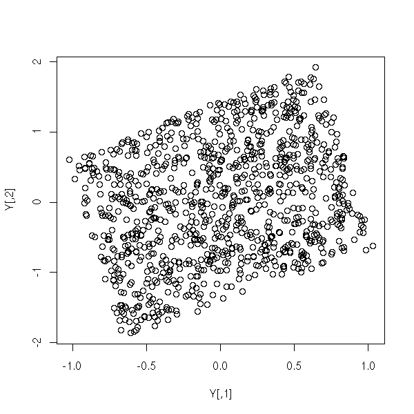
Let us see on an example how it differs with Principal Component Analysis: let us take two random variables X1 and X2, uniformly distributed
N <- 1000
X <- matrix(runif(2*N, -1, 1), nc=2)
plot(X)
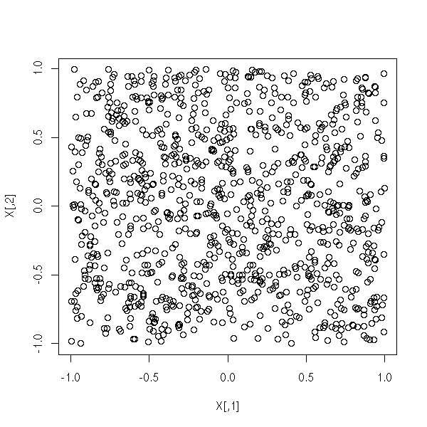
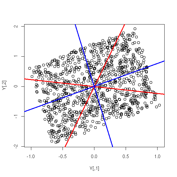
and transform them
M <- matrix(rnorm(4), nc=2)
Y <- X %*% M
plot(Y)
We get a parallelogram. PCA would yield something close to its largest diagonal (red, in the following plot); ICA would yield the image of the axes (blue), i.e., new axes parallel to the sides of the parallelogram.
plot(Y)
p <- prcomp(Y)$rotation
abline(0, p[2,1] / p[1,1], col="red", lwd=3)
abline(0, -p[1,1] / p[2,1], col="red", lwd=3)
abline(0, M[1,2]/M[1,1], col="blue", lwd=3)
abline(0, M[2,2]/M[2,1], col="blue", lwd=3)
Other examples:
op <- par(mfrow=c(2,2), mar=c(1,1,1,1))
for (i in 1:4) {
  N <- 1000
  X <- matrix(runif(2*N, -1, 1), nc=2)
  M <- matrix(rnorm(4), nc=2)
  Y <- X %*% M
  plot(Y, xlab="", ylab="")
  p <- prcomp(Y)$rotation
  abline(0, p[2,1] / p[1,1], col="red", lwd=3)
  abline(0, -p[1,1] / p[2,1], col="red", lwd=3)
  abline(0, M[1,2]/M[1,1], col="blue", lwd=3)
  abline(0, M[2,2]/M[2,1], col="blue", lwd=3)
}
par(op)
The ICA yields the variables that were indeed used.
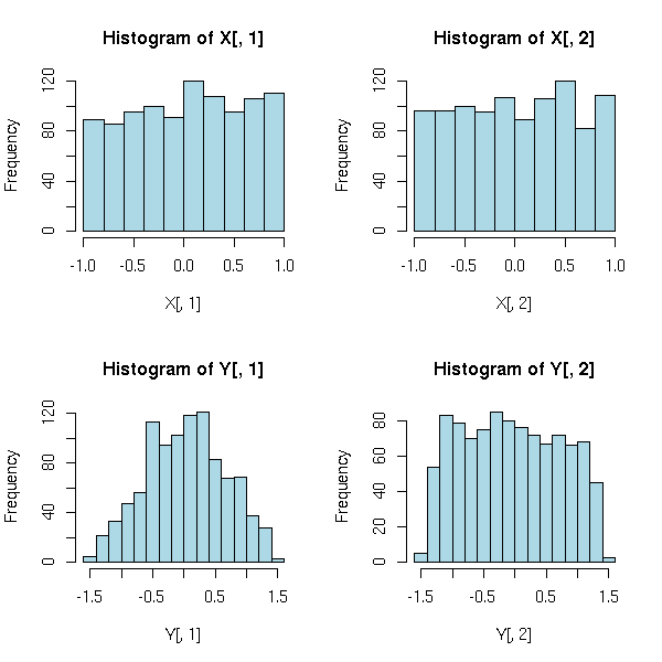
The main idea behind the algorithm is the fact that (from the central limit theorem) a linear combination of non-gaussian random variables is "more gaussian".
op <- par(mfrow=c(2,2))
hist(X[,1], col="light blue")
hist(X[,2], col="light blue")
hist(Y[,1], col="light blue")
hist(Y[,2], col="light blue")
par(op)
Therefore the algorithm goes as follows:
1. Normalize the data, so that they have a variance equal
   to 1 and that the be uncorrelated.
2. Find (with the usual numeric optimization algorithms)
   the linear transformation that maximizes the
   non-gaussianity.
To this end, one can use several measures of non-gaussianity: the kurtosis (i.e., the fourth moment), the entropy (integral of -f * log(f), where f is the pdf), mutual information, etc.
There are two implementations of this algorithm in R. The first one, "ica" in the "e1071" package, does not give the expected results.
library(e1071)
r <- ica(Y,.1)
plot(r$projection)

The second one, "mlica" in the "mlica" package, gives the expected result.
library(mlica)
ICA <- function (x,...) {
   prPCA <- PriorNormPCA(x);
   prNCP <- proposeNCP(prPCA,0.1);
   mlica(prNCP,...)
}

set.seed(1) # It sometimes crashes...
N <- 1000
X <- matrix(runif(2*N, -1, 1), nc=2)
M <- matrix(rnorm(4), nc=2)
Y <- X %*% M
r <- ICA(Y)
plot(r$S)
TODO: Give more interesting results.
See also:
http://www.cis.hut.fi/projects/ica/icademo/
http://www.cs.helsinki.fi/u/ahyvarin/papers/NN00new.pdf
Principal Component Analysis is about approximating a variance matrix. The simplest approximation is a scalar matrix (a diagonal matrix with always the same element on the diagonal), the next simplest is a diagonal matrix; then comes the PCA, which writes the variance matrix as V = B B' for some rectangular matrix B, with as many columns as you want components. The matrix B can be characterized as the matrix that minimizes the norm of V - B B' (actually, it is not unique, but (a.s.) unique up to multiplication by an orthogonal matrix). The next step is the factor model: we write V as B B' + Delta, where Delta is a diagonal matrix.
In R, this is obtained with the factanal() function.
r <- factanal(covmat = V, factors = k)
# The correlation matrix
v <- r$loadings %*% t(r$loadings) + diag(r$uniquenesses)
# The corresponding variance matrix
v <- diag(sqrt(diag(V))) %*% v %*% diag(sqrt(diag(V)))
This is used, for instance, in finance: we model stock returns as a multidimensional gaussian distribution. A portfolio can be seen as a linear combination of stocks; the coefficients are called the weights of the portfolio and are usually assumed to sum up to 1 (you might also want them to be positive). If w is a portfolio and V the variance matrix of the distribution of returns, then the returns of the portfolio are gaussian with variance w' V w; the square root of this variance is called the risk of the portfolio. Finding the portfolio with the minimum risk possible sounds simple enough (it is an optimization problem), but you have to estimate the variance matrix in the first place. If your universe contains thousands of stocks, you actually want to estimate a 1000*1000 matrix: you will never have enough data to do that! You need a way to reduce the number of quantities to estimate, you need a way to more parsimoniously parametrize variance matrices. Principal Component Analysis is the classical way of doing this, but it assumes that all the stocks respond to the same few sources of randomness: this is not a reasonable assumption. Instead, we assume that the stocks respond to a few "risk factors" (they could be interpreted as, e.g., oil prices, comsumption indexes, interest rates, etc.) and an idiosyncratic component, specific to each stock: this is a factor model. Such an estimation of the variance matrix of stock returns is called a risk model.
TODO: An example with actual computations (portfolio optimization?)
TODO: Merge this section with the previous

TODO: Decide whether to put this section here or together with the
variance matrix (there is already a note about RMT somewhere)...
Principal Component analysis can also be seen as decomposition of a variance matrix, that can also lead to a simplification of variance matrices (by discarding the eigenvectors with low eigenvalues), to a parametrization of variance matrices with few parameters. Since large variance matrices require a huge amount of data to be reliably estimated, PCA can allow you to get a precise (but biased) estimation with little data.
Those parametrizations are often called "factor models". They are used, for instance, in finance: when you want to invest in stocks (or any other asset, actually), you do not buy the stocks for which you have a positive view in equal quantities: some of those stocks can be moving together. Consider for instance three stocks, A, B and C, on which you have a positive view, where A and B tend to mode together and C moves independently from A and B: it might not be a good idea to invest a third of your wealth in each of them -- it might be wiser to invest half in C, and a quarter in A and B. This reasoning can be formalized (and justified) if one assumes that the returns of those three assets follow a gaussian distribution with mean (mu, mu, mu) (where mu is the expected return of those assets -- here we assume they are equal) and correlation matrix
 1  1/2  0
1/2  1   0
 0   0   1
We want to find the portfolio (i.e., the combination of assets) with the lowest risk, i.e., the lowest variance.
But where do we get this variance matrix in the first place? We have to estimate it with historical data: for instance from the monthly returns of the stocks in the past three years. But if you have 1000 stocks (that is a small number: in real life, it is usually between 1000 and 10,000), that is 36,000 data points to estimate around 500,000 parameters -- this is not reasonable.
The idea is to assume that the variance matrix has some simple form, i.e., that it can be parametrized with a reasonable number of parameters. For instance, one can assume that the correlations between the returns is due to their being correlated with a small number of "factors": then, we just have to give the "exposure" of the each stock to each factor, B and the variance matrix of the factors, v. The variance matrix of the stock returns is then
V = B v B'
If one assumes that the factors are independant (and of variance 1), i.e., their variance matrix is the identity matrix, v=1, and V = B B'.
But this is very similar to the decomposition of a variance matrix provided by PCA: if, furthermore, we do not know the factors beforehand, we can simply select them as the first eigenvectors.
This is called a noiseless statistical factor model.
TODO: Noiseless factor model
TODO: Scalar factor model
TODO: Approximate factor model
TODO: The double Procrustes problem?
When the data you are modeling are functions (for instance, the evolution over time of some quantity), you might realize that the principal components are noisy and try to smooth them. Actually, this is not the optimal thing to do -- by smoothing the principal components, you run the risk of smoothing away the information they were supposed to contain. Instead, you can put the smoothing inside the PCA algorithm.
The first step is usually to express the functions to be studied in some basis -- by doing so, you already smooth them, but you should be careful not to discard the features of interest. Using functions instead of series of points allows you to have a different number of points, a different sampling frequency for each curve -- or even, irregular sampling. Using a basis of functions brings the problem back in the finite-dimensional realm and reduces it to a linear algebra problem.
In the second step, one computes the mean of all those curves, usually using the same basis.
TODO: Do we add a smoothing penalty for the mean?
TODO: Formula...
In the third step, one actually performs the principal component analysis.
TODO: Explain how to introduce the smoothing penalties
TODO: Formulas
TODO: Implementation?
A few problems might occur.
For instance, the functions to estimate might have some very important properties: for instance, we might know that they have to be increasing, in spite of error measurements. We can enforce such a requirement by parametrizing the function via a differential equation. For instance, to get an increasing function H (say, height, when studying child growth), one just has to find a function w (without any restriction) such that H'' = w H -- w can be interpreted as the "relative acceleration".
Another problem is that the features in the various curves to study are not aligned: they occur in the same order, but with different amplitudes and locations. In that situation, the mean curve can fail to exhibit the very features we want to study -- they are averaged out. To palliate this problem, one can "align" the curves, by reparametrizing the curves (i.e., by considering an alternate time: clock time versus physiological time in biology, clock time versus market time or transaction time in finance, etc.). This is called "registration" or "(dynamic) time warping".
TODO: More details on time warping.

TODO:
1. Write the functions to study in some basis
2. Smoothed mean
3. Smoothed PCA
For more details, check:
Applied Functional Data Analysis, Methods and Case Studies
J.O. Ramsay and B.W. Silverman, Springer Verlag (2002)
http://www.stats.ox.ac.uk/~silverma/fdacasebook/

TODO: An online reference?
The components you get as the result of a principal component analysis are not always directly interpretable: even if all the relevant information is in the first two principal components, they are not as "pure" as you would like. But by rotating them, they can be easier to interpret. Since you use the amplitude of the loadings of the PCA to interpret the principal components, you can try to simplify them, as follows: find a rotation (not a rotation of the whole space, but only a rotation of the subspace spanned by the first components) that maximizes the variance of the loadings (contrary to PCA, you do not consider the components one at a time, but all at the same time). This will actually try to make the loadings either very large or very small, easing the interpretation of the components.
?varimax
?promax
When you apply Principal Component Analysis (PCA) to the pixels of a series of images, you forget the 2-dimensional structure and hope that the PCA will somehow recover it, by itself. Instead, one can try to retain that information by representing the data as matrices. This can be generalized to higher-dimensional data with higher dimensional arrays (learned people may call those arrays "tensors").
Tensor algebra, motivations:
- Taylor expansion f(x+h) = f(x) + f'(x).h + f''(x).h.h + ...
  where f(x)   is a number
        f'(x)  is a 1-form: it transforms a vector h into
                            a number f'(x).h
        f''(x) is a symetric 2-form: it takes a two
                            vectors h and k and turns them
                            into a number f''(x).h.k
- Higher order statistics (HOS) (e.g., the autocorrelation
  of x^2 is a fourth moment).
- [For category-theorists] The tensor algebra TV of a
  vector space V is obtained from the adjoint of the
  forgetful functor Alg --> Vect from the category of
  R-algebras to that of R-vector spaces. Similarly, one can
  define the symetric tensor algebra SV from the category of
  commutative R-algebras. The alternating algebra AV is
  often defined as AV=TV/SV.
- In mathematical physics, a tensor is a section of some
  vector bundle built from the tangent buldle of a
  manifold (if you do not know about manifolds, read "The
  large scale structure of space-time" by S. Hawking et
  al.). For instance:
    - a section of the tangent bundle TX --> X is a field of
      tangent vectors;
    - a section of the cotangent bundle (the dual of the
      tangent space) TX' --> X is a (field of) 1-forms;
    - a section of the maximum alternating power of the
      cotangent bundle is an n-form, that you can use to
      integrate a (real-valued) function on the manifold.
  (You can also consider sections of other vector bundles,
  e.g., the Levi-Civita connection -- some people call
  those "holors" -- see "Theory of Holors : A Generalization
  of Tensors", P. Moon and E. Spencer)
Tentative implementation:
# From "Out-of-code tensor approximation of
# multi-dimensional matrices of visual data"
# H. Wang et al., Siggraph 2005
# http://vision.ai.uiuc.edu/~wanghc/research/siggraph05.html
# http://vision.ai.uiuc.edu/~wanghc/papers/siggraph05_tensor_hongcheng.pdf
mode.n.vector <- function (A, n) { # aka "unfolding"
  stopifnot( n == floor(n),
             n >= 1,
             n <= length(dim(A)) )
  res <- apply(A, n, as.vector)
  if (is.vector(res)) {
    res <- matrix(res, nr=dim(A)[n], nc=prod(dim(A))/dim(A)[n] )
  } else {
    res <- t(res)
  }
  stopifnot( dim(res) == c( dim(A)[n], prod(dim(A))/dim(A)[n] ) )
  res
}
n.rank <- function (A, n) {
  sum( svd( mode.n.vector(A, n) )$d
       >= 1000 * .Machine$double.eps )
}
n.ranks <- function (A) {
  n <- length(dim(A))
  res <- integer(n)
  for (i in 1:n) {
    res[i] <- n.rank(A, i)
  }
  res
}
# The norm is the same as usual: sqrt(sum(A^2))
n.mode.svd <- function (A) {
  res <- list()
  for (n in 1:length(dim(A))) {
    res[[n]] <- svd( mode.n.vector(A, n) )
  }
  res
}
product <- function (A, B, i) {
  # Multiply the ith dimension of the tensor A with the
  # columns of the matrix B
  stopifnot( is.array(A),
             i == floor(i),
             length(i) == 1,
             i >= 1,
             i <= length(dim(A)),
             is.matrix(B),
             dim(A)[i] == dim(B)[1]
           )
  res <- array( apply(A, i, as.vector) %*% B,
                dim = c(dim(A)[-i], dim(B)[2]) )
  N <- length(dim(A))
  ind <- 1:N
  ind[i] <- N
  ind[ 1:N > i ] <- ind[ 1:N > i ] - 1
  res <- aperm(res, ind)
  stopifnot( dim(res)[-i] == dim(A)[-i],
             dim(res)[i]  == dim(B)[2] )
  res
}

# A few tests...
A <- array(1:8, dim=c(2,2,2))
mode.n.vector(A, 1)
mode.n.vector(A, 2)
mode.n.vector(A, 3)
n.rank(A, 1)
n.rank(A, 2)
n.rank(A, 3)
n.ranks(A)

B1 <- matrix(round(10*rnorm(6)),  nr=2, nc=3)
B2 <- matrix(round(10*rnorm(12)), nr=3, nc=4)
all( product(B1, B2, 2) == B1 %*% B2 )

# The main function...
tensor.approximation <- function (A, R) {
  stopifnot( is.array(A),
             length(dim(A)) == length(R),
             is.vector(R),
             R == floor(R),
             R >= 0,
             R <= dim(A),
             R <= n.ranks(A),
             R <= prod(R)/R    # If all the elements of R
                               # are equal, this is fine.
           )
  N <- length(R)
  I <- dim(A)
  U <- list()
  for (i in 1:N) {
    U[[i]] <- matrix( rnorm(I[i] * R[i]), nr = I[i], nc = R[i] )
  }
  finished <- FALSE
  BB <- NULL
  while (!finished) {
    cat("Iteration\n")
    Utilde <- list()
    for (i in 1:N) {
      Utilde[[i]] <- A
      for (j in 1:N) {
        if (i != j) {
          Utilde[[i]] <- product( Utilde[[i]], U[[j]], j)
        }
        cat("  Utilde[[", i, "]]: ",
            paste(dim(Utilde[[i]]),collapse=","),
            "\n", sep="")
      }
      stopifnot( length(dim(Utilde[[i]])) == N,
                 dim(Utilde[[i]])[i] == dim(A)[i],
                 dim(Utilde[[i]])[-i] == R[-i] )
      Utilde[[i]] <- mode.n.vector( Utilde[[i]], i )
      cat("  Utilde[[", i, "]]: ",
          paste(dim(Utilde[[i]]),collapse=","),
          "\n", sep="")
    }
    for (i in 1:N) {
      U[[i]] <- svd( Utilde[[i]] ) $ u [ , 1: R[i], drop=FALSE ]
      #U[[i]] <- svd( Utilde[[i]] ) $ v
      stopifnot( dim(U[[i]]) == c(I[i], R[i]) )
    }
    B <- A
    for (j in 1:N) {
      B <- product( B, U[[j]], j )
    }
    res <- B
    for (j in 1:N) {
      res <- product( res, t(U[[j]]), j )
    }
    cat("Approximating A:", sum((res - A)^2), "\n")
    if (!is.null(BB)) {
      eps <- sum( (B - BB)^2 )
      cat("Improvement on B:", eps, "\n")
      finished <- eps <= 1e-6
    }
    BB <- B
  }
  res <- B
  for (j in 1:N) {
    res <- product( res, t(U[[j]]), j )
  }
  attr(res, "B") <- B
  attr(res, "U") <- U
  attr(res, "squared.error") <- sum( (A-res)^2 )
  res
}
A <- array(1:24, dim=c(4,3,2))
x <- tensor.approximation(A, c(1,1,1))
x <- tensor.approximation(A, c(2,2,2))
The problem is now the following: given a set of points in an n-dimensional space, find their coordinates kwnowing only their distances. Usually, you do not know the space dimension either.
This is very similar to Principal Component Analysis (PCA), with a few differences, though: PCA looks for relations between the variables while PCO focuses on similarities between the observations; you can interpret the PCA axes with the variables while you cannot with PCO (indeed, there are no variables).
As PCA, PCO is linear and the computations are the same: in PCA, we start with the variance-covariance matrix, i.e., a matrix whose entries are sums of squares; in distance analysis, we consider a matrix of distances or a distance of squares of matrices, i.e., from the pythagorean theorem, a matrix of sums of squares.
In other words, PCO is just PCA without its first step: the computation of the variance-covariance (or "squared distances") matrix.
?cmdscale
library(MASS)
MDS is a non-linear equivalent of Principal Coordinate Analysis (PCO). We have a set of distances between points and we try to assign coordinates to those points so as to minimize a "stress function" -- for instance, the sum of squares between the distances we have and the distances obtained from the coordinates.
There are several R functions to perform those computations.
?cmdscale             Principal coordinate analysis (metric, linear)
library(MASS)
?sammon               (metric, non-linear)
?isoMDS               (non-metric)
There was a comparison of them in RNews:
http://cran.r-project.org/doc/Rnews/Rnews_2003-3.pdf
library(xgobi)
?xgvis

TODO: speak a little more of xgvis
xgvis slides and tutorial:
http://industry.ebi.ac.uk/%257Ealan/VisWorkshop99/XGvis_Talk/sld001.htm
http://industry.ebi.ac.uk/%257Ealan/VisWorkshop99/XGvis_Tutorial/index.html
(restart the MDS optimization with a different starting point to
avoid local minima ("scramble" button))
(one may change the parameters (euclidian/L1/Linfty distance,
removal of outliers, weights, etc.)
(one may ask for a 3D or 4D layout and the rotate it in xgobi)
(restart the MDS optimization with only a subset of the data --
interactivity)
What is a Shepard diagram ??? (change the power transformation)
MDS to get a picture of protein similarity
MDS warning: The global shape of MDS configurations is determined by
the large dissimilarities; consequently, small distances should be
in terpreted with caution: they may not reflect small
dissimilarities.
The applications are manifold, for instance:
1. Dimension reduction: we start with a set of points in a high-dimensional space, compute their pairwise distances, and try to put the points in a space of smaller dimension while retaining as much as possible the information ("proximity") present in the distance matrix.
Thus, we can see MDS as a non-linear analogue of Principal Component Analysis (PCA).
n <- 100
v <- .1
# (Almost) planar data
x <- rnorm(n)
y <- x*x + v*rnorm(n)
z <- v*rnorm(n)
d <- cbind(x,y,z)
# A rotation
random.rotation.matrix <- function (n=3) {
  m <- NULL
  for (i in 1:n) {
    x <- rnorm(n)
    x <- x / sqrt(sum(x*x))
    y <- rep(0,n)
    if (i>1) for (j in 1:(i-1)) {
      y <- y + sum( x * m[,j] ) * m[,j]
    }
    x <- x - y
    x <- x / sqrt(sum(x*x))
    m <- cbind(m, x)
  }
  m
}
m <- random.rotation.matrix(3)
d <- t( m %*% t(d) )
pairs(d)
title(main="The points lie in a plane")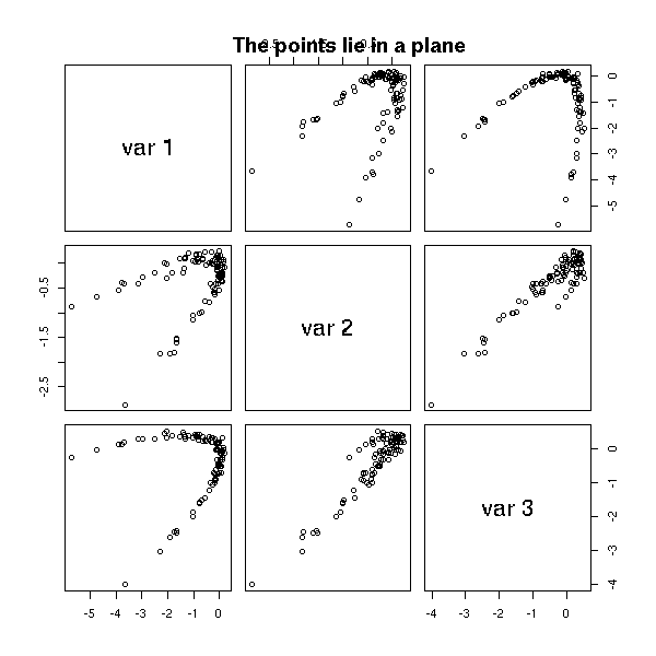
pairs(cmdscale(dist(d),3))
title(main="MDS")

pairs(princomp(d)$scores)
title(main="Principal Component Analysis")

2. Study of data with no coordinates, for instance protein similarity: we can tell when two proteins are similar, we can quantify this similarity -- but we have no coordinates, we cannot think of a simple vector space whose points could be interpreted as proteins. MDS can help build such a space and graphically represent the proximity relations among a set of proteins.
The same process also appears in psychology: we can ask test subjects to identify objects (faces, Morse-coded letters, etc.) and count the number of confusions between two objects. This measures the similarity of these objects (a subjective similarity, that stems from their representation in the human mind); MDS can assign coordinates to those objects and represent those similarities in a graphical way.
Those misclassifications also appear in statistics: we can use MDS to study forecast errors of a given statistical algorithm (logistic regression, neural nets, etc.) when trying to predict a qualitative variable from quantitative variables.
TODO: speak about MDS when I tackle those algorithms...
3. MDS can also graphically represent variables (and not observations), after estimating the "distances" between variables from their correlations.
TODO: such a plot when I speak about variable selection...
4. We can also use MDS to plot graphs (the combinatorial objects we study in graph theory -- see the "graph" package), described by theiir vertices and edges.
Alternatively, you can use GraphViz,
http://www.graphviz.org/
outside R or from R -- see the "sem" and "Rgraphviz" libraries.
TODO
5. Reconstruct a molecule, especially its shape, from the distance between its atoms.
For more details, see
http://www.research.att.com/areas/stat/xgobi/papers/xgvis.ps.gz
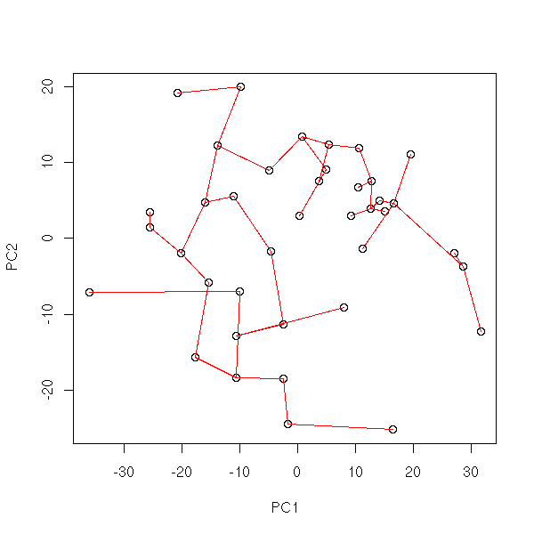
1. Put the points into 4 or 5 classes (e.g., by hierarchical
classification, or with the k-means algorithm).
2. Take the median point of those classes.
3. Is the Minimum Spanning Tree (MST) of those points ramified?
On our examples:
# Data
n <- 200  # Number of patients, number of columns
k <- 10   # Dimension of the ambient space
nb.points <- 5
p <- matrix( 5*rnorm(nb.points*k), nr=k )
barycentre <- function (x, n) {
  # Add number between the values of x in order to get a length n vector
  i <- seq(1,length(x)-.001,length=n)
  j <- floor(i)
  l <- i-j
  (1-l)*x[j] + l*x[j+1]
}
m <- apply(p, 1, barycentre, n)
data.broken.line <- t(m)
data.noisy.broken.line <- data.broken.line + rnorm(length(data.broken.line))
library(splines)
barycentre2 <- function (y,n) {
  m <- length(y)
  x <- 1:m
  r <- interpSpline(x,y)
  #r <- lm( y ~ bs(x, knots=m) )
  predict(r, seq(1,m,length=n))$y
}
data.curve <- apply(p, 1, barycentre2, n)
data.curve <- t(data.curve)
data.noisy.curve <- data.curve + rnorm(length(data.curve))
data.real <- read.table("Tla_z.txt", sep=",")
r <- prcomp(t(data.real))
data.real.3d <- r$x[,1:3]

library(cluster)
library(ape)
mst.of.classification <- function (x, k=6, ...) {
  x <- t(x)
  x <- t( t(x) - apply(x,2,mean) )
  r <- prcomp(x)
  y <- r$x
  u <- r$rotation
  r <- kmeans(y,k)
  z <- r$centers
  m <- mst(dist(z))
  plot(y[,1:2], ...)
  points(z[,1:2], col='red', pch=15)
  w <- which(m!=0)
  i <- as.vector(row(m))[w]
  j <- as.vector(col(m))[w]
  segments( z[i,1], z[i,2], z[j,1], z[j,2], col='red' )
}
set.seed(1)
mst.of.classification(data.curve, 6)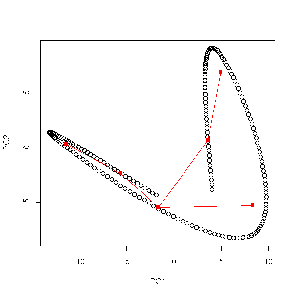
mst.of.classification(data.curve, 6)

op <- par(mfrow=c(2,2),mar=.1+c(0,0,0,0))
for (k in c(4,6,10,15)) {
  mst.of.classification(data.curve, k, axes=F)
  box()
}
par(op)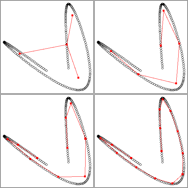
op <- par(mfrow=c(2,2),mar=.1+c(0,0,0,0))
for (k in c(4,6,10,15)) {
  mst.of.classification(data.noisy.curve, k, axes=F)
  box()
}
par(op)
op <- par(mfrow=c(2,2),mar=.1+c(0,0,0,0))
for (k in c(4,6,10,15)) {
  mst.of.classification(data.broken.line, k, axes=F)
  box()
}
par(op)
op <- par(mfrow=c(2,2),mar=.1+c(0,0,0,0))
for (k in c(4,6,10,15)) {
  mst.of.classification(data.noisy.broken.line, k, axes=F)
  box()
}
par(op)
With real data, it does not work that well:
op <- par(mfrow=c(2,2),mar=.1+c(0,0,0,0))
for (k in c(4,6,10,15)) {
  mst.of.classification(data.real, k, axes=F)
  box()
}
par(op)
Details:
op <- par(mfrow=c(3,3),mar=.1+c(0,0,0,0))
for (k in c(4:6)) {
  for (i in 1:3) {
    mst.of.classification(data.real, k, axes=F)
    box()
  }
}
par(op)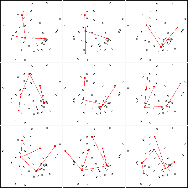
op <- par(mfrow=c(3,3),mar=.1+c(0,0,0,0))
for (k in c(7:9)) {
  for (i in 1:3) {
    mst.of.classification(data.real, k, axes=F)
    box()
  }
}
par(op)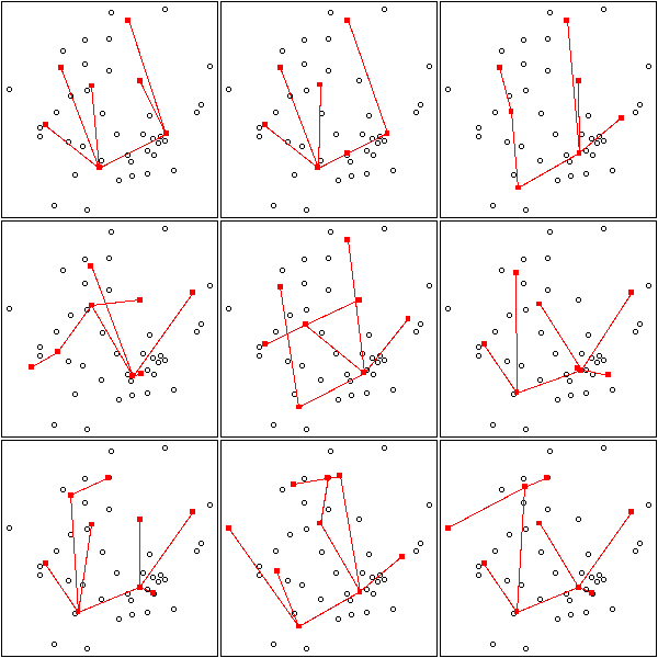
op <- par(mfrow=c(3,3),mar=.1+c(0,0,0,0))
for (k in c(10:12)) {
  for (i in 1:3) {
    mst.of.classification(data.real, k, axes=F)
    box()
  }
}
par(op)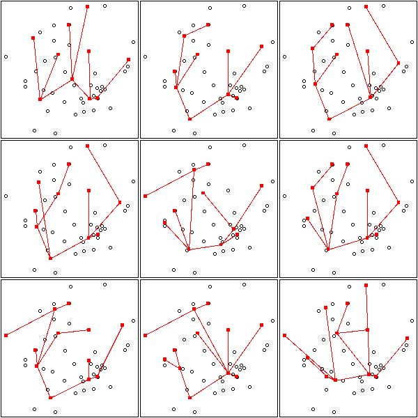
op <- par(mfrow=c(3,5),mar=.1+c(0,0,0,0))
for (k in c(13:15)) {
  for (i in 1:3) {
    mst.of.classification(data.real, k, axes=F)
    box()
  }
}
par(op)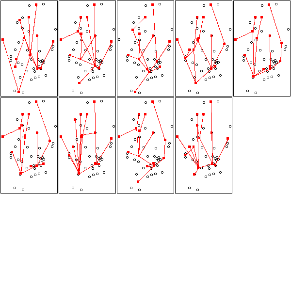
library(ape)
my.plot.mst <- function (d) {
  r <- mst(dist(t(d)))
  d <- prcomp(t(d))$x[,1:2]
  plot(d)
  n <- dim(r)[1]
  w <- which(r!=0)
  i <- as.vector(row(r))[w]
  j <- as.vector(col(r))[w]
  segments( d[i,1], d[i,2], d[j,1], d[j,2], col='red' )
}
my.plot.mst(data.broken.line)
my.plot.mst(data.noisy.broken.line)
my.plot.mst(data.curve)
my.plot.mst(data.noisy.curve)

my.plot.mst(data.real)

my.plot.mst(t(data.real.3d))
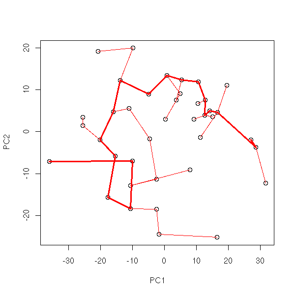
Pruned MST
# Gives the list of the oaths from the branching nodes to the leaves
chemins.vers.les.feuilles <- function (G) {
  nodes <- which(apply(G,2,sum)>2)
  leaves <- which(apply(G,2,sum)==1)
  res <- list()
  for (a in nodes) {
    for (b in which(G[a,]>0)) {
      if (! b %in% nodes) {
        res <- append(res,list(c(a,b)))
      }
    }
  }
  chemins.vers.les.feuilles.suite(G, nodes, leaves, res)
}
# Last coordinate of a vector
end1 <- function (x) {
  n <- length(x)
  x[n]
}
# Last two coordinates of a vector
end2 <- function (x) {
  n <- length(x)
  x[c(n-1,n)]
}
chemins.vers.les.feuilles.suite <- function (G, nodes, leaves, res) {
  new <- list()
  done <- T
  for (ch in res) {
    if( end1(ch) %in% nodes ) {
      # Pass
    } else if ( end1(ch) %in% leaves ) {
      new <- append(new, list(ch))
    } else {
      done <- F
      a <- end2(ch)[1]
      b <- end2(ch)[2]
      for (x in which(G[b,]>0)) {
        if( x != a ){
          new <- append(new, list(c( ch, x )))
        }
      }
    }
  }
  if(done) {
    return(new)
  } else {
    return(chemins.vers.les.feuilles.suite(G,nodes,leaves,new))
  }
}

G <- matrix(c(0,1,0,0, 1,0,1,1, 0,1,0,0, 0,1,0,0), nr=4)
chemins.vers.les.feuilles(G)

# Compute the length of a path
longueur.chemin <- function (chemin, d) {
  d <- as.matrix(d)
  n <- length(chemin)
  i <- chemin[ 1:(n-1) ]
  j <- chemin[ 2:n ]
  if (n==2) {
    d[i,j]
  } else {
    sum(diag(d[i,][,j]))
  }
}

G <- matrix(c(0,1,0,0, 1,0,1,1, 0,1,0,0, 0,1,0,0), nr=4)
d <- matrix(c(0,2,4,3, 2,0,2,1, 4,2,0,3, 3,1,3,0), nr=4)
chemins <- chemins.vers.les.feuilles(G)
chemins
l <- sapply(chemins, longueur.chemin, d)
l
stopifnot( l == c(2,2,1) )

elague <- function (G0, d0) {
  d0 <- as.matrix(d0)
  G <- G0
  d <- d0
  res <- 1:dim(d)[1]
  chemins <- chemins.vers.les.feuilles(G)
  while (length(chemins)>0) {
    longueurs <- sapply(chemins, longueur.chemin, d)
    # Number of the shortest path
    i <- which( longueurs == min(longueurs) )[1]
    cat(paste("Removing", paste(res[chemins[[i]]],collapse=' '), "length =", longueurs[i],"\n"))
    # Nodes to remove
    j <- chemins[[i]] [-1]
    res <- res[-j]
    G <- G[-j,][,-j]
    d <- d[-j,][,-j]
    cat(paste("Removing", paste(j), "\n" ))
    cat(paste("", paste(res, collapse=' '), "\n"))
    chemins <- chemins.vers.les.feuilles(G)
  }
  res
}

library(ape)
my.plot.mst <- function (x0) {
  cat("Plotting the points\n")
  x <- prcomp(t(x0))$x[,1:2]
  plot(x)
  cat("Computing the distance matrix\n")
  d <- dist(t(x0))
  cat("Computing the MST (Minimum Spanning Tree)\n")
  G <- mst(d)
  cat("Plotting the MST\n")
  n <- dim(G)[1]
  w <- which(G!=0)
  i <- as.vector(row(G))[w]
  j <- as.vector(col(G))[w]
  segments( x[i,1], x[i,2], x[j,1], x[j,2], col='red' )
  cat("Pruning the tree\n")
  k <- elague(G,d)
  cat("Plotting the pruned tree\n")
  x <- x[k,]
  G <- G[k,][,k]
  n <- dim(G)[1]
  w <- which(G!=0)
  i <- as.vector(row(G))[w]
  j <- as.vector(col(G))[w]
  segments( x[i,1], x[i,2], x[j,1], x[j,2], col='red', lwd=3 )
}

my.plot.mst(data.noisy.broken.line)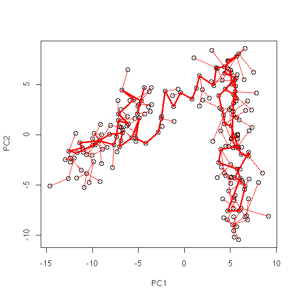
my.plot.mst(data.noisy.curve)
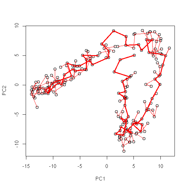
my.plot.mst(data.real)

my.plot.mst(t(data.real.3d))
Remark: in image analysis, we sometimes us a simplification of this algorithm (still called "pruning" to get rid of the ramifications in the skeleton of an image: we just gnaw two of three segments from each leaf.
TODO: a reference
TODO: reference
TODO: explain
Let us first construct the graph.
# k: each point is linked to its k nearest neighbors
# eps: each point is linked to all its neighbors within a radius eps
isomap.incidence.matrix <- function (d, eps=NA, k=NA) {
stopifnot(xor( is.na(eps), is.na(k) ))
d <- as.matrix(d)
if(!is.na(eps)) {
im <- d <= eps
} else {
im <- apply(d,1,rank) <= k+1
diag(im) <- F
}
im | t(im)
}
plot.graph <- function (im,x,y=NULL, ...) {
if(is.null(y)) {
y <- x[,2]
x <- x[,1]
}
plot(x,y, ...)
k <- which( as.vector(im) )
i <- as.vector(col(im))[ k ]
j <- as.vector(row(im))[ k ]
segments( x[i], y[i], x[j], y[j], col='red' )
}
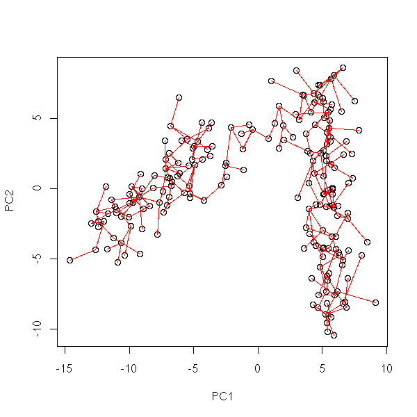
d <- dist(t(data.noisy.curve))
r <- princomp(t(data.noisy.curve))
x <- r$scores[,1]
y <- r$scores[,2]
plot.graph(isomap.incidence.matrix(d, k=5), x, y)
So far, there is a problem: the resulting grah need not be connected -- this is a problem if we want to compute distances...
plot.graph(isomap.incidence.matrix(d, eps=quantile(as.vector(d), .05)),
           x, y)
The graph is connected if and only if it contains the Minimum Spanning Tree (MST): thus, we shall just add the edges of this MST taht are not already there.
isomap.incidence.matrix <- function (d, eps=NA, k=NA) {
  stopifnot(xor( is.na(eps), is.na(k) ))
  d <- as.matrix(d)
  if(!is.na(eps)) {
    im <- d <= eps
  } else {
    im <- apply(d,1,rank) <= k+1
    diag(im) <- F
  }
  im | t(im) | mst(d)
}
plot.graph(isomap.incidence.matrix(d, eps=quantile(as.vector(d), .05)),
           x, y)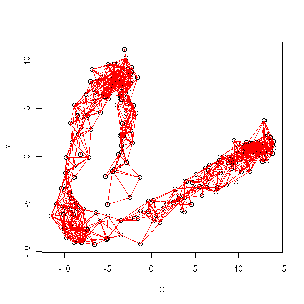
TODO: distance in this graph. It is a classical problem: shortest path in a graph.
inf <- function (x,y) { ifelse(x<y,x,y) }
isomap.distance <- function (im, d) {
d <- as.matrix(d)
n <- dim(d)[1]
dd <- ifelse(im, d, Inf)
for (k in 1:n) {
dd <- inf(dd, matrix(dd[,k],nr=n,nc=n) + matrix(dd[k,],nr=n,nc=n,byrow=T))
}
dd
}
isomap <- function (x, d=dist(x), eps=NA, k=NA) {
im <- isomap.incidence.matrix(d, eps, k)
dd <- isomap.distance(im,d)
r <- list(x,d,incidence.matrix=im,distance=dd)
class(r) <- "isomap"
r
}
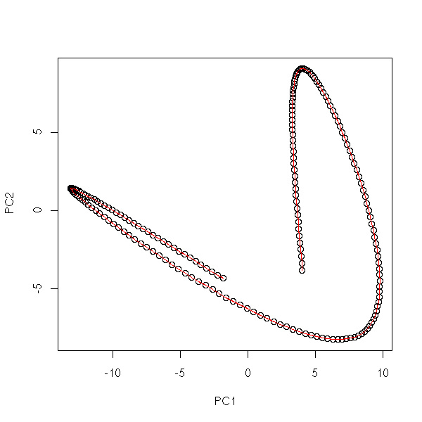
r <- isomap(t(data.noisy.curve), k=5)
xy <- cmdscale(r$distance,2) # long: around 30 seconds
plot.graph(r$incidence.matrix, xy)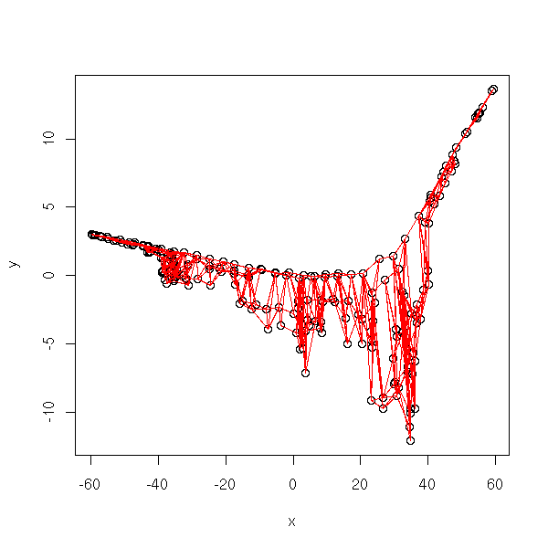
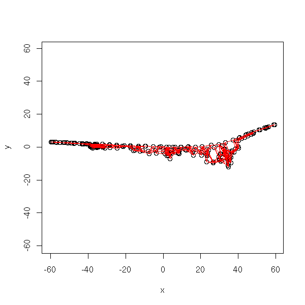
In an orthonormal basis:
plot.graph(r$incidence.matrix, xy, ylim=range(xy))
TODO:
Other ways of representing the results:
1. Initial data, graph
2. MDS
3. Initial coordinates, graph, colors for the first coordinate of
   the MDS.
4. The curve?
TODO: apply this to our data.
TODO: Choosing the parameters (eps or k)
Kohonen networks (or SOM, Self-Organizing Maps) are a qualitative, non-linear equivalent of Principal Component (or Coordinate) Analysis (PCA, PCO): we try to classify observations in several classes (unknown classes) and to organize those classes into a spacial layout. For instance, we can want the classes to be aligned:
* * * * * * * * * *
or to form a grid:
*  *  *  *  *  *  *  *  *  *

*  *  *  *  *  *  *  *  *  *

*  *  *  *  *  *  *  *  *  *

*  *  *  *  *  *  *  *  *  *

*  *  *  *  *  *  *  *  *  *

*  *  *  *  *  *  *  *  *  *
We start with a cloud of points in an n-dimensional space, whose coordinates will be written (x1,x2,...,xi,...,xn) and we try to find, for each element j of the grid, coordinates (w(1,j),w(2,j),...,w(i,j),...,w(n,j)).
In other words, we try to embed the grid in this n-dimensional space, so that it comes as close as possible to the points (as if the points were magnetic and were attracting the grid vertices) and so that it retains its grid shape (as if the grid edges were springs).
1. Choose random values for the w(i,j).
2. Take a point x = (x1,...,xn) in the cloud.
2a. Consider the point j on the gris whose coordinates are the closest from x:
j = ArgMin Sum(  (x_i - w(i,j))^2  )
            i
2b. Compute the error vector:
d_i = x_i - w(i,j)
2c. For each point k of the grid in the neighbourhood of j, replace the value of w(i,k):
w(i,k) <- w(i,k) + h * d_i.
3. Go back to point 2, with a smaller neighbourhood and a smaller value for the learning coefficient h.
You can replace the notion of neighbourhood by a "neighbourhood function":
w(i,k) <- w(i,k) + h * v(i,k) * d_i
where v(i,i) = 1 and v(i,k) decreases when k goes away from i. Iteration after iteration, you will replace the function one with a more and more visible peak.
You can choose the grid geometry: often, a table of dimension 1, 2 or 3, but it could also be a circle, a cylinder, a torus, etc.
In that sense, we can say that Kohonen networks are non-linear (a would be tempted to say "homotopically non-linear").
You can also interpret Kohonen networks as a mixture of Principal Component Analysis (finding a graphical representation, in the plane, of a cloud of points) and unsupervised classification (assign the points to classes, a priori unknown).
You can assess the quality of the result by looking at the error, i.e., the average of the
Sum(  (x_i - w(i,j))^2  )
 i
when x runs over the points to classify and where j is the class that minimizes this sum (i.e., j is the class to which x_i is assigned):
MSE = Mean Min Sum  (x_i - w(i,j))^2
        x   j   i
Kohonen networks are often presented as a special case of neural networks: if the doodles used to explain them are similar, trying hard to see a neural network in a Kohonen network might slow your understanding of the subject (the weights are completely different, there is no transfer function, etc.).
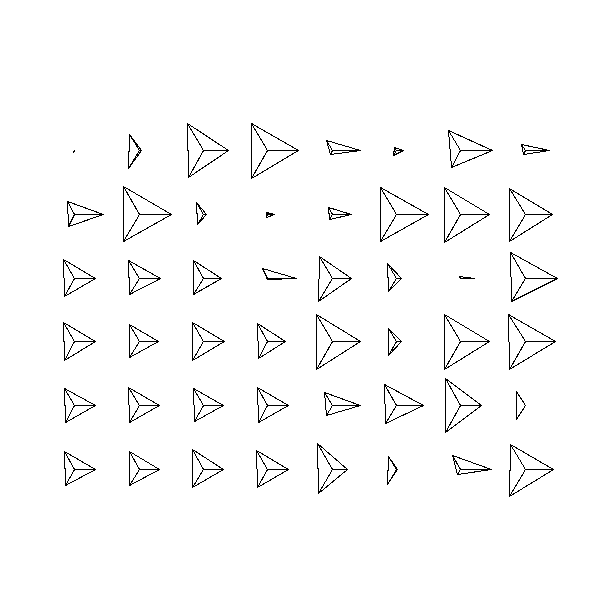
You can plot each class j by a disc or a square, and put, in each square, its coordinates w(1,j),...,w(n,j), as a star plot or as a parallel plot.
Under R, there are two functions to compute Kohonen maps, in the "class" and "som" packages (if you hesitate, choose "som").
The following examples use a Kohonen map to describe the palette (i.e., the colors) of an image (this is supposed to be a landscape: an island in the middle of a river).

library(pixmap)
x <- read.pnm("photo1.ppm")
d <- cbind( as.vector(x@red),
            as.vector(x@green),
            as.vector(x@blue) )
m <- apply(d,2,mean)
d <- t(  t(d) - m )
s <- apply(d,2,sd)
d <- t(  t(d) / s )
library(som)
r1 <- som(d,5,5)
plot(r1)
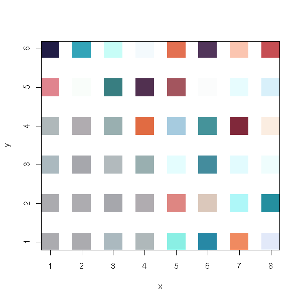
x <- r1$code.sum$x
y <- r1$code.sum$y
n <- r1$code.sum$nobs
co <- r1$code   # Is it in the same order that x, y and n?
co <- t( t(co) * s + m )
plot(x, y,
     pch=15,
     cex=5,
     col=rgb(co[,1], co[,2], co[,3])
    )
x <- r1$code.sum$x
y <- r1$code.sum$y
n <- r1$code.sum$nobs
co <- r1$code   # Is it in the same order that x, y and n?
co <- t( t(co) * s + m )
plot(x, y,
     pch=15,
     cex=5*n/max(n),
     col=rgb(co[,1], co[,2], co[,3])
    )
library(class)
r2 <- SOM(d)
plot(r2)
x <- r2$grid$pts[,1]
y <- r2$grid$pts[,2]
n <- 1   # Where???
co <- r2$codes
co <- t( t(co) * s + m )
plot(x, y,
     pch=15,
     cex=5*n/max(n),
     col=rgb(co[,1], co[,2], co[,3])
    )
You will notice that the result is not always the same:
op <- par(mfrow=c(2,2))
for (i in 1:4) {
  r2 <- SOM(d)
  plot(r2)
}
par(op)
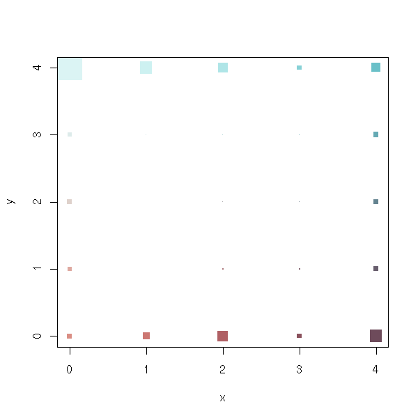
You may want to plot the vertex coordinates: you can use one colour per coordinate. This allows you to graphically choose which variables to use: you can eliminate those that play little role in the classification and those that bring the same information as already selected variables.
In the first example, the first coordinate is informative (it coincides with one of the map coordinates). The two others contain the same information (we can get rid of one) and correspond to a diagonal direction on the map.
x <- r1$code.sum$x
y <- r1$code.sum$y
v <- r1$code

op <- par(mfrow=c(2,2), mar=c(1,1,1,1))
for (k in 1:dim(v)[2]) {
  m <- matrix(NA, nr=max(x), nc=max(y))
  for (i in 1:length(x)) {
    m[ x[i], y[i] ] <- v[i,k]
  }
  image(m, col=rainbow(255), axes=F)
}
par(op)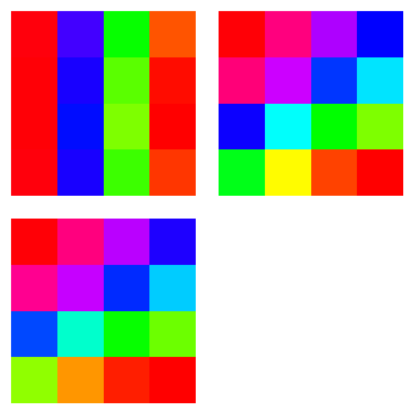
x <- r2$grid$pts[,1]
y <- r2$grid$pts[,2]
v <- r2$codes

op <- par(mfrow=c(2,2), mar=c(1,1,1,1))
for (k in 1:dim(v)[2]) {
  m <- matrix(NA, nr=max(x), nc=max(y))
  for (i in 1:length(x)) {
    m[ x[i], y[i] ] <- v[i,k]
  }
  image(m, col=rainbow(255), axes=F)
}
par(op)
The vertex coordinates define a map from the plane (the space in which the Kohonen map lives) towards R^n (the space in which our cloud of points lives): we can plot this application (or, more precisely, its image), especially when the space R^n is of low dimension -- if the dimension is high, you would resort to high-dimensional visualization tools, such as ggobi.
TODO: plot
TODO: shards plot, to represent the differences between a
cell and its neighbours.

library(klaR)
?shardsplot
TODO: sammon plot, to see how distorted the map is.
TODO: colouring a SOM; one can use another, 1-dimensional, SOM to choose the colours (it can be a colour ring or a colour segment).
One can plot the grid and visualize how well it fits the cloud of points using a grand tour -- for instance, using ggobi.
Image analysis (medicine: echography, etc.; handwriting): an n*m image can be seen as a point an an n*m-dimensional space. The euclidian distance is not the most adequate one, but it works pretty well nonetheless.
You can also use Kohonen maps to forecast time series: usually, we try to write
y[n+1] = f( y[n], y[n-1], ..., y[n-k] )
for a "well-chosen" k and a map f to be determined (for example, by a linear regression, a non-linear regression, a Principal Component Analysis (PCA), a Curvilinear Component Analysis (CCA), etc.). Instead of this, you can build a Kohonen map with ( y[n], y[n-1], ..., y[n-k] ) and look at the values of y[n+1] at each vertex of the map. You could also use ( y[n+1], y[n], y[n-1], ..., y[n-k] ) to build the map.
TODO: develop this example, either here or in the Time
Series chapter
You can use Kohonen maps to measure the colours in an image (for instance, to convertr it from 16 bits to 8 bits, or to convert it to an indexedd format, that limits the number of colors but lets you choose those colours): the vertex coordinates will be the quantified colors.
http://www.cis.hut.fi/~lendasse/pdf/esann00.pdf
You can also use Kohonen maps for supervised learning: you still start with a cloud of points, but this time, each point already belongs to a class -- in other words, we have quantitative predictive variables, as before, and a further qualitative variable, to predict/explain.
We run the algorithm on the predictive variables and we associate one (or several) class(es) to each node of the map: the classes of a node are the classes of the points it contains. Vertices with several classes are in a "clash state".
The interest is twofold: first, you can use the mao to predict the class of new observations, second, you get a graphical representation of the qualitative variable to predict, i.e., you have a notion of proximity, similarity, between the classes.
We said above that Kohonen maps were not very stable: it you change a few points in the cloud of points, or simply if you change the initialization of the map, you get completely different results.
However, small maps (3x3) are rather stable -- actually, the fact is more general: unsupervised learning methods give reproducible results up to 10 classes, but not above.
However, you can simplify a large Kohonen map in the following way: if you colour the map vertices with the number of points it contains, you can apply image processing algorithms (mathematical morphology), such as the opening (to get rid of noise, i.e., small elements) or the watershed (that divides the image in several bassins of attraction).
TODO: translate the last word...

TODO: what about the hierarchical algorithm: a 3x3 SOM,
then a 3x3 SOM in each of its cells, etc.?  Do I mention
it later?
You can model the situation described by a SOM (i.e., simulate data that will be efficiently analyzed by a SOM) as follows. To get a cloud of points:
1. Take a point at random in the plane, following some distribution. One of the aims of the SOM algorithm is to recover this distribution.
2. Apply a transformation (one other aim of the SOM distribution is to recover this transformation) to send our point in an n-dimensional space. Our point is then on a 2-dimensional submanifold (a submanifold is like a subspace, but it need not be "straight", it may be "curved") of R^n.
3. Add some noise.
The Kohonen map is an estimation of the distribution of the first step: the rows and columns correspond to the coordinates in the plane; the number of points in each vertex is an estimation of the density.
The coordinates w(i,j) of the vertices are an estimation of the submanifold in step 2.
In those estimations, the plane R^2 and the submanifold of R^n have been discretized.
Generative Topographic Mappings (GTM) are a possible replacement of SOM that formalize this geometric description of Kohonen maps.
http://research.microsoft.com/~cmbishop/downloads/Bishop-GTM-Ncomp-98.pdf
TODO: introduction
TODO: proofread the following paragraph.
The following methods are all based on principal component analysis: we start with a table of numbers (the values of our variables for PCA, a contingency table for CA), we consider its columns as points in an n-dimensional space (same for the rows), and we look for the 2-dimensional subspace of R^n (the space in which the columns live -- and we would do the same for that in which the rows live) on which we can see "as much information as possible" (we project the cloud of points onto it, orthogonally with respect to the canonical scalar product or another scalar product, more appropriate to the problem at hand.
Correspondance analysis focuses on contingency tables, i.e., qualitative variables. Let us first consider the case of two variables.
TODO: recall what a contingency table is...
We first transform the contingency table into two tables: that of row-profiles (the sum of the elements in a row is always 1 (or 100%)) and that of column-profiles.
TODO: define f(i,*) and f(*,j)
If the two variables are independant, we have f(i,j)=f(i,*)f(*,j). You can use Pearson's Chi^2 test to compare the distributions of f(i,j) and f(i,*)f(*,j).
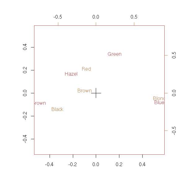
From a technical point of vue, Correspondance Analysis analysis looks like Principal Component Analysis. We try to find a graphical representation of the rows and colums of the table, as points in some space; we want the points to reflect the information contained in the table as faithfully as possible (technically, we try to maximize the variance of the resulting cloud of points). Correspondance Analysis proceeds in a similar way, the only difference being that the distance is not given by the canonical scalar product but is the "Chi^2 distance".
library(MASS)
data(HairEyeColor)
x <- HairEyeColor[,,1]+HairEyeColor[,,2]
biplot(corresp(x, nf = 2))
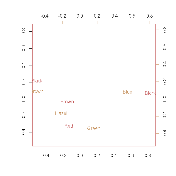
biplot(corresp(t(x), nf = 2))
# ???
plot(corresp(x, nf=1))

If there are more variables, we can add them, a posteriori, on the plot, with the predict.mca function.
Other examples
n <- 100
m <- matrix(sample(c(T,F),n^2,replace=T), nr=n, nc=n)
biplot(corresp(m, nf=2), main="Correspondance Analysis of Random Data")

vp <- corresp(m, nf=100)$cor
plot(vp, ylim=c(0,max(vp)), type='l',
     main="Correspondance Analysis of Random Data")
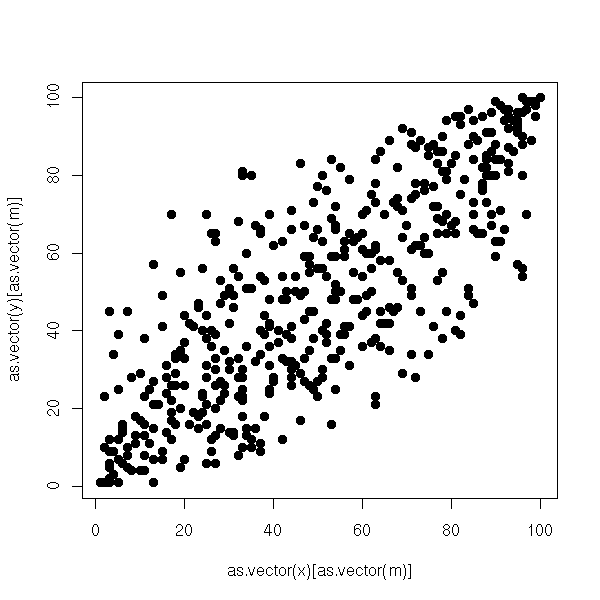
n <- 100
x <- matrix(1:n, nr=n, nc=n, byrow=F)
y <- matrix(1:n, nr=n, nc=n, byrow=T)
m <- abs(x-y) <= n/10
biplot(corresp(m, nf=2),
       main='Correspondance Analysis of "Band" Data')
vp <- corresp(m, nf=100)$cor
plot(vp, ylim=c(0,max(vp)), type='l',
       main='Correspondance Analysis of "Band" Data')
You can also check the "ca" function.
library(multiv)
?ca
We start with a table, containing 0s and 1s, with a very simple form
n <- 100
x <- matrix(1:n, nr=n, nc=n, byrow=F)
y <- matrix(1:n, nr=n, nc=n, byrow=T)
m <- abs(x-y) <= n/10
plot.boolean.matrix <- function (m) { # Voir aussi levelplot
  nx <- dim(m)[1]
  ny <- dim(m)[2]
  x <- matrix(1:nx, nr=nx, nc=ny, byrow=F)
  y <- matrix(1:ny, nr=nx, nc=ny, byrow=T)
  plot( as.vector(x)[ as.vector(m) ], as.vector(y)[ as.vector(m) ], pch=16 )
}
plot.boolean.matrix(m)
But someone changed (or forgot to give us) the order of the rows and columns -- if the data is experimental, we might not have any a priori clue as to the order.
ox <- sample(1:n, n, replace=F)
oy <- sample(1:n, n, replace=F)
reorder.matrix <- function (m,ox,oy) {
  m <- m[ox,]
  m <- m[,oy]
  m
}
m2 <- reorder.matrix(m,ox,oy)
plot.boolean.matrix(m2)
We can reorder rows and columns as follows:
a <- corresp(m2)
o1 <- order(a$rscore)
o2 <- order(a$cscore)
m3 <- reorder.matrix(m2,o1,o2)
plot.boolean.matrix(m3)

Had we started with random data, the result could have been:
n <- 100
p <- .05
done <- F
while( !done ){
  # We often get singular matrices
  m2 <- matrix( sample(c(F,T), n*n, replace=T, prob=c(1-p, p)), nr=n, nc=n )
  done <- det(m2) != 0
}
plot.boolean.matrix(m2)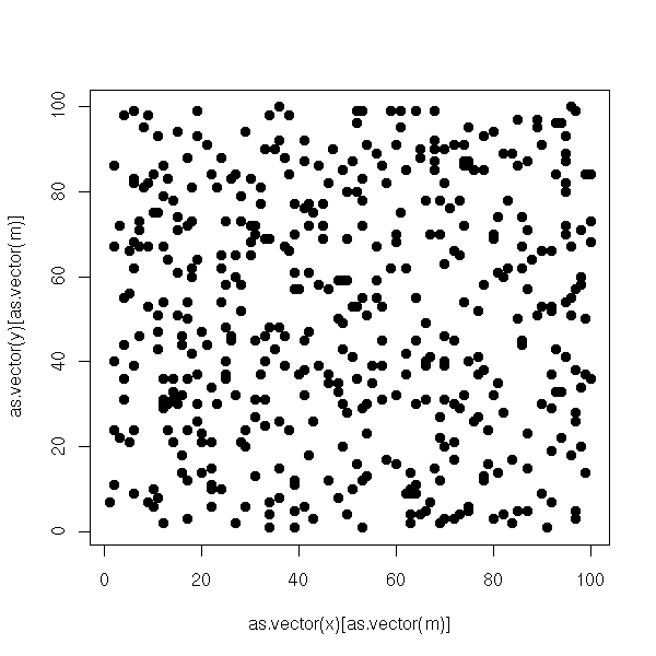
a <- corresp(m2)
o1 <- order(a$rscore)
o2 <- order(a$cscore)
m3 <- reorder.matrix(m2,o1,o2)
plot.boolean.matrix(m3)
The idea is very simple. We start with a contingency table (for two qualitative variables), we transform it into a frequency table, we compute the marginal frequencies and the frequencies we would have had if the two variables had been independant, we compute the difference, so as to get a "centered" matrix, that describes the lack of independance of the two variables. We then perform a Principal Component Analysis, but not with the canonical distance: instead, we use a weighted distance between row-profiles (resp. column-profiles) so that each column (resp. row) have the same importance. This is called the Chi^2 distance.
# Euclidian Distance
sum ( f_{i,j} - f_{i',j} )^2

# Euclidian distance between the row-profiles
       f_{i,j}     f_{i',j}
sum ( --------- - ---------- )^2
 j     f_{i,.}     f_{i',.}

# Chi^2 distance
        1       f_{i,j}     f_{i',j}
sum --------- ( --------- - ---------- )^2
 j   j_{.,j}    f_{i,.}     f_{i',.}
We choose this metric because it has the following property: we can group some values of a variable without changing the result. (For instance, we could replace one of the two variables, X, whose values are A, B, C, D, E, F, by another variable X' with values A, BC, D, E, F, in the obvious way, if we think that the differences between B and C are not that relevant.)
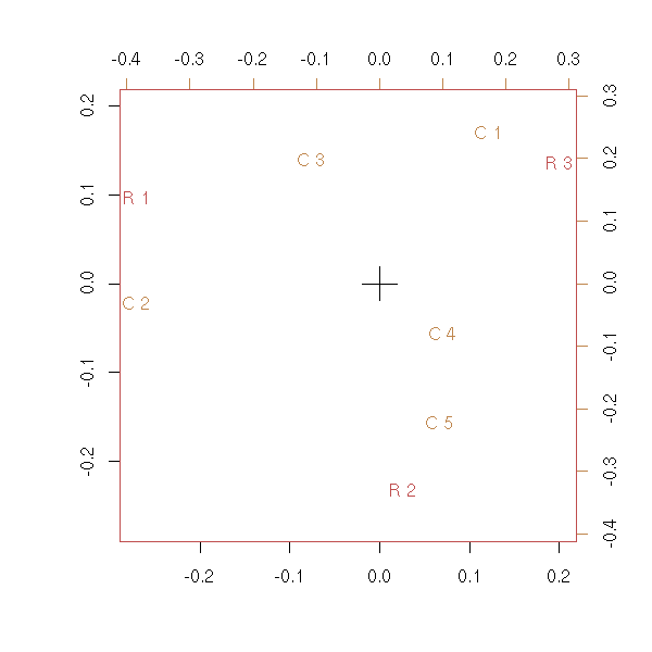
# Correspondance Analysis
my.ac <- function (x) {
  if(any(x<0))
    stop("Expecting a contingency matrix -- with no negative entries")
  x <- x/sum(x)
  nr <- dim(x)[1]
  nc <- dim(x)[2]
  marges.lignes <- apply(x,2,sum)
  marges.colonnes <- apply(x,1,sum)
  profils.lignes <- x / matrix(marges.lignes, nr=nr, nc=nc, byrow=F)
  profils.colonnes <- x / matrix(marges.colonnes, nr=nr, nc=nc, byrow=T)
  # Do not forget to center the matrix: we compute the frequency matrix
  # we would have if the variables were independant and we take the difference.
  x <- x - outer(marges.colonnes, marges.lignes)
  e1 <- eigen( t(x) %*% diag(1/marges.colonnes) %*% x %*% diag(1/marges.lignes) )
  e2 <- eigen( x %*% diag(1/marges.lignes) %*% t(x) %*% diag(1/marges.colonnes) )
  v.col <- solve( e2$vectors, x )
  v.row <- solve( e1$vectors, t(x) )
  v.col <- t(v.col)
  v.row <- t(v.row)
  if(nr<nc)
    valeurs.propres <- e1$values
  else
    valeurs.propres <- e2$values
  # Dessin
  plot( v.row[,1:2],
        xlab='', ylab='', frame.plot=F )
  par(new=T)
  plot( v.col[,1:2], col='red',
        axes=F, xlab='', ylab='', pch='+')
  axis(3, col='red')
  axis(4, col='red')
  # Return the data
  invisible(list(donnees=x, colonnes=v.col, lignes=v.row,
                 valeurs.propres=valeurs.propres))
}

nr <- 3
nc <- 5
x <- matrix(rpois(nr*nc,10), nr=nr, nc=nc)
my.ac(x)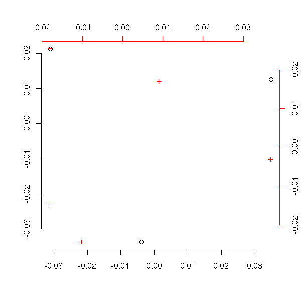
Let us compare our result with that of the "corresp" function.
plot(corresp(x,nf=2))
Exercice: Modify the code above so that it uses the "svd" function instead of "eigen" (this is a real problem: as the matrix is no longer symetric, numeric computations can yield non-real eigen values).
On the plot representing the first variable, we can add the points corresponding to the second: we just take the barycenters of the first points, weighted by the corresponding (row- or column-) profile. We can do the same thing of the plot for the second variable: up to the scale, we should get the same result -- it is this property that justifies the superposition of both plots.
TODO: both plots
The barycenter also allows us to add new variables to the plots.
TODO
library(CoCoAn)
library(multiv)
library(ade4)
Simple Correspondance Analysis tackled the problem of two qualitative variables; multiple correspondance analysis caters to more than two variables. Usually, the data are not given as a contingency matrix (or "hypermatrix": if there are n variables, it should be an n-dimensional table), because this matrix would have a huge number of elements, most of them null. We use a table similar to that used to quantitative variables:
    Hair   Eye    Sex
1  Blond  Blue   Male
2  Brown Brown Female
3  Brown  Blue Female
4    Red Brown   Male
5    Red Brown Female
6  Brown Brown Female
7  Brown Brown Female
8  Black Brown   Male
9  Brown  Blue Female
10 Blond  Blue   Male
...
Here is the example from the manual.
library(MASS)
data(farms)
farms.mca <- mca(farms, abbrev=TRUE)
farms.mca
plot(farms.mca)
Let us consider again the eye and hair colour data set. As the data are given by a contingency hypermatrix, we first have to transform it.
# Not pretty
my.table.to.data.frame <- function (a) {
  r <- NULL
  d <- as.data.frame.table(a)
  n1 <- dim(d)[1]
  n2 <- dim(d)[2]-1
  for (i in 1:n1) {
    for (j in 1:(d[i,n2+1])) {
      r <- rbind(r, d[i,1:n2])
    }
    row.names(r) <- 1:dim(r)[1]
  }
  r
}
r <- my.table.to.data.frame(HairEyeColor)
plot(mca(r))
We can also add mor subjects or variables, afterwards, with the "predict.mca" function.
?predict.mca
If there are only two variables, we can perform a simple or multiple correspondance analysis: the result is not exactly the same, but remains very similar.
x <- HairEyeColor[,,1]+HairEyeColor[,,2]
op <- par(mfcol=c(1,2))
biplot(corresp(x, nf = 2),
       main="Simple Correspondance Analysis")
plot(mca(my.table.to.data.frame(x)), rows=F,
     main="Multiple Correspondance Analysis")
par(op)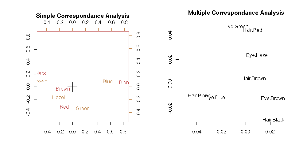
We first transform the data, to turn it into a "disjunctive table":
      HairBlack HairBrown HairRed HairBlond EyeBrown EyeBlue EyeHazel EyeGreen SexMale SexFemale
 [1,]         0         0       0         1        0       1        0        0       1         0
 [2,]         0         1       0         0        1       0        0        0       0         1
 [3,]         0         1       0         0        0       1        0        0       0         1
 [4,]         0         0       1         0        1       0        0        0       1         0
 [5,]         0         0       1         0        1       0        0        0       0         1
 [6,]         0         1       0         0        1       0        0        0       0         1
 [7,]         0         1       0         0        1       0        0        0       0         1
 [8,]         1         0       0         0        1       0        0        0       1         0
 [9,]         0         1       0         0        0       1        0        0       0         1
[10,]         0         0       0         1        0       1        0        0       1         0
Then we do an "analysis" (this term is used to describe the common part of the PCA, CA, MCA algorithms): the observations all have the same weight, the variables are weighted as for Simple Correspondance Analysis. We remark that 1 is always an eigenvalue: we shall remove the corresponding vector.
TODO: explain where this "1" comes from and explain why we remove it.

It comes from the fact that we did not center the data:

We have a cloud of points, not centered, and we try to find a line
through the origin that "fits" the cloud as tightly as
possible. This is the line through the center of gravity of the
cloud. It is not relevant (it does not really depend on the cloud of
points, but rather on the position of the origin), so we discard
it.
Here is a bit of code that performs that kind of computation.
# Multiple Correspondance Analysis
tableau.disjonctif.vecteur <- function (x) {
  y <- matrix(0, nr=length(x), nc=length(levels(x)))
  for (i in 1:length(x)) {
    y[i, as.numeric(x[i])] <- 1
  }
  y
}
tableau.disjonctif <- function (x) {
  if( is.vector(x) )
    y <- tableau.disjonctif.vecteur(x)
  else {
    y <- NULL
    y.names <- NULL
    for (i in 1:length(x)) {
      y <- cbind(y, tableau.disjonctif.vecteur(x[,i]))
      y.names <- c( y.names, paste(names(x)[i], levels(x[,i]), sep='') )
    }
  }
  colnames(y) <- y.names
  y
}
my.acm <- function (x, garder.un=F) {
  # x is a data.frame that contains only factors
  # y is a boolean matrix (it only contains 0s and 1s)
  y <- tableau.disjonctif(x)
  # Number of observations
  n <- dim(y)[1]
  # Number of variables
  s <- length(x)
  # Number of columns in the disjunctive table
  p <- dim(y)[2]
  # The matrix and the weights
  F <- y/(n*s)
  Dp <- diag(t(y)%*%y) / (n*s)
  Dn <- rep(1/n,n)
  # Let us perform the analysis
  # Do NOT forget to remove 1 as an eigenvalue!!!
  # (it comes from the fact that we did not center the matrix)
  e1 <- eigen( t(F) %*% diag(1/Dn) %*% F %*% diag(1/Dp) )
  e2 <- eigen( F %*% diag(1/Dp) %*% t(F) %*% diag(1/Dn) )
  variables <- t(e2$vectors) %*% F
  individus <- t(e1$vectors) %*% t(F)
  variables <- t(variables)
  individus <- t(individus)
  valeurs.propres <- e1$values
  if( !garder.un ) {
    variables <- variables[,-1]
    individus <- individus[,-1]
    valeurs.propres <- valeurs.propres[-1]
  }
  plot( jitter(individus[,2], factor=5) ~ jitter(individus[,1], factor=5),
        xlab='', ylab='', frame.plot=F )
  par(new=T)
  plot( variables[,1:2], col='red',
        axes=FALSE, xlab='', ylab='', type='n' )
  text( variables[,1:2], colnames(y), col='red')
  axis(3, col='red')
  axis(4, col='red')
  j <- 1
  col = rainbow(s)
  for (i in 1:s) {
    jj <- j + length(levels(x[,i])) - 1
    print( paste(j,jj) )
    lines( variables[j:jj,1], variables[j:jj,2], col=col[i] )
    j <- jj+1
  }
  invisible(list( donnees=x, variables=variables, individus=individus,
                  valeurs.propres=valeurs.propres ))
}

random.data.1 <- function () {
  n <- 100
  m <- 3
  l <- c(3,2,5)
  x <- NULL
  for (i in 1:m) {
    v <- factor( sample(1:l[i], n, replace=T), levels=1:l[i] )
    if( is.null(x) )
      x <- data.frame(v)
    else
      x <- data.frame(x, v)
  }
  names(x) <- LETTERS[1:m]
  x
}
r <- NULL
while(is.null(r)) {
  x1 <- random.data.1()
  try(r <- my.acm(x1))
}
On the preceding plot, the three variables are well separated, a telltale sign that they are independant. Here is what happens if they are dependant.
my.random.data.2 <- function () {
  n <- 100
  m <- 3
  l <- c(3,2,3)
  x <- NULL
  for (i in 1:m) {
    v <- factor( sample(1:l[i], n, replace=T), levels=1:l[i] )
    if( is.null(x) )
      x <- data.frame(v)
    else
      x <- data.frame(x, v)
  }
  x[,3] <- factor( ifelse( runif(n)>.8, x[,1], x[,3] ), levels=1:l[1])
  names(x) <- LETTERS[1:m]
  x
}
r <- NULL
while(is.null(r)) {
  x2 <- my.random.data.2()
  try(r <- my.acm(x2))
}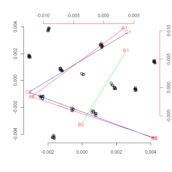
Let us compare our result with that of the "mca" command.
library(MASS)
plot(mca(x1))

plot(mca(x2))
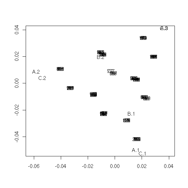
At first, I had forgotten to remove the 1 eigenvalue, and I got this.
my.acm(x1, garder.un=T)

my.acm(x2, garder.un=T)
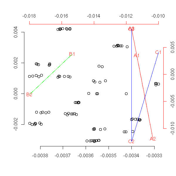
(What follows are a few mindless tests -- none actually worked.)
One could try to analyse a set of qualitative and quantitative variables by mixing Principal Component Analysis (PCA) and Multiple Correspondance Analysis (MCA): we just put the two tables side by side and concatenate the weight vectors of the columns. Let us look at the results.
tableau.disjonctif.vecteur <- function (x) {
  if( is.factor(x) ){
    y <- matrix(0, nr=length(x), nc=length(levels(x)))
    for (i in 1:length(x)) {
    y[i, as.numeric(x[i])] <- 1
    }
    return(y)
  } else
  return(x)
}
tableau.disjonctif <- function (x) {
  if( is.vector(x) )
    y <- tableau.disjonctif.vecteur(x)
  else {
    y <- NULL
    y.names <- NULL
    for (i in 1:length(x)) {
      y <- cbind(y, tableau.disjonctif.vecteur(x[,i]))
      if( is.factor(x[,i]) )
        y.names <- c( y.names, paste(names(x)[i], levels(x[,i]), sep='') )
      else
        y.names <- c(y.names, names(x)[i])
    }
  }
  colnames(y) <- y.names
  y
}
my.am <- function (x) {
  y <- tableau.disjonctif(x)
  # Number of observations
  n <- dim(y)[1]
  # Number of variables
  s <- length(x)
  # Number of columns of the disjunctive table
  p <- dim(y)[2]

  # The matrix and the weights
  # Each variable weight is 1, but for the qualitative variables
  # that are "split" into several "subvariables", it is the sum of
  # those "subvariable" weights that is 1.
  Dp <- diag(t(y)%*%y) / n
  j <- 1
  for(i in 1:s){
    if( is.factor(x[,i]) )
      j <- j + length(levels(x[,i]))
    else {
      Dp[j] <- 1
      j <- j+1
    }
  }
  Dn <- rep(1,n)
  # It if not a good idea to center the variable...
  f <- ne.pas.centrer(y)
  # We perform the analysis...
  e1 <- eigen( t(f) %*% diag(1/Dn) %*% f %*% diag(1/Dp) )
  e2 <- eigen( f %*% diag(1/Dp) %*% t(f) %*% diag(1/Dn) )
  variables <- t(e2$vectors) %*% f
  individus <- t(e1$vectors) %*% t(f)
  variables <- t(variables)
  individus <- t(individus)
  valeurs.propres <- e1$values
  # Sometimes, because of rounding errors, the matrix becomes
  # non-diagonalizable in R. We then end up with complex eigenvalues
  # and (worse) complex eigenvectors. That is why it is a better
  # idea to use the SVD, that always yields real results.
  if( any(Im(variables)!=0) | any(Im(individus)!=0) |
      any(Im(valeurs.propres)!=0) ){
    warning("Matrix not diagonalizable on R!!!")
    variables <- Re(variables)
    individus <- Re(individus)
    valeurs.propres <- Re(valeurs.propres)
  }
  plot( jitter(individus[,2], factor=5) ~ jitter(individus[,1], factor=5),
        xlab='', ylab='', frame.plot=F )
  par(new=T)
  plot( variables[,1:2], col='red',
        axes=FALSE, xlab='', ylab='', type='n' )
  text( variables[,1:2], colnames(y), col='red')
  axis(3, col='red')
  axis(4, col='red')
  col = rainbow(s)
  j <- 1
  for (i in 1:s) {
    if( is.factor(x[,i]) ){
      jj <- j + length(levels(x[,i])) - 1
      print( paste(j,jj) )
      lines( variables[j:jj,1], variables[j:jj,2], col=col[i] )
      j <- jj+1
    } else {
      arrows(0,0,variables[j,1],variables[j,2],col=col[i])
      j <- j+1
    }
  }
}
ne.pas.centrer <- function (y) { y }

n <- 500
m <- 3
p <- 2
l <- c(3,2,5)
x <- NULL
for (i in 1:m) {
  v <- factor( sample(1:l[i], n, replace=T), levels=1:l[i] )
  if( is.null(x) )
    x <- data.frame(v)
  else
    x <- data.frame(x, v)
}
x <- cbind( x, matrix( rnorm(n*p), nr=n, nc=p ) )
names(x) <- LETTERS[1:(m+p)]
x1 <- x
my.am(x1)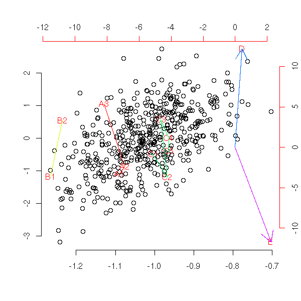
If the variables are dependant, we can see that the qualitative variables are linked (as with multiple correspondance analysis), but there is nothing obvious with the quantitative variable...
n <- 500
m <- 3
p <- 2
l <- c(3,2,5)
x <- NULL
for (i in 1:m) {
  v <- factor( sample(1:l[i], n, replace=T), levels=1:l[i] )
  if( is.null(x) )
    x <- data.frame(v)
  else
    x <- data.frame(x, v)
}
x <- cbind( x, matrix( rnorm(n*p), nr=n, nc=p ) )
names(x) <- LETTERS[1:(m+p)]
x[,3] <- factor( ifelse( runif(n)>.8, x[,1], x[,3] ), levels=1:l[1])
x[,5] <- scale( ifelse( runif(n)>.9, as.numeric(x[,1]), as.numeric(x[,2]) )) + .1*rnorm(n)
x2 <- x
my.am(x2)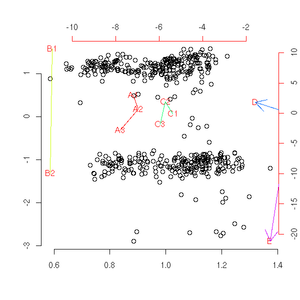
If we center the matrix, the results are meaningless (however, we can center the columns for the quantitative variables).
ne.pas.centrer <- function (y) {
  centre <- apply(y, 2, mean)
  y - matrix(centre, nr=n, nc=dim(y)[2], byrow=T)
}
my.am(x1)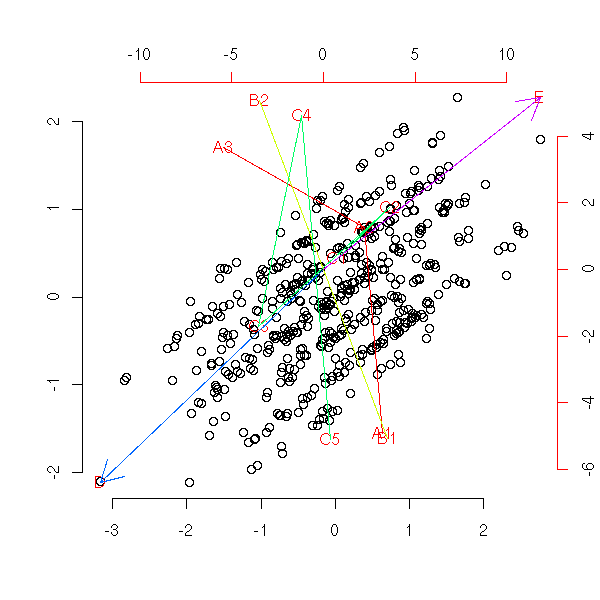
my.am(x2)

To plot, on the same graph, qualitative and quantitative variables, a simple solution is to turn the quantitative variables into qualitative variables.
People will tell you that this is always a bad idea: you lose "some" information. And indeed, there is not much to be seen: this is rather unhelpful...
to.factor.numeric.vector <- function (x, number) {
  resultat <- NULL
  intervalles <- co.intervals(x,number,overlap=0)
  for (i in 1:number) {
    if( i==1 ) intervalles[i,1] = min(x)
    else
      intervalles[i,1] <- intervalles[i-1,2]
    if( i==number )
      intervalles[i,2] <- max(x)
  }
  for (valeur in x) {
    r <- NA
    for (i in 1:number) {
      if( valeur >= intervalles[i,1] & valeur <= intervalles[i,2] )
        r <- i
    }
    resultat <- append(resultat, r)
  }
  factor(resultat, levels=1:number)
}
to.factor.vector <- function (x, number) {
  if( is.factor(x) )
    return(x)
  else
    return(to.factor.numeric.vector(x,number))
}
to.factor <- function (x, number=4 ) {
  y <- NULL
  for (a in x) {
    aa <- to.factor.vector(a, number)
    if( is.null(y) )
      y <- data.frame(aa)
    else
      y <- data.frame(y,aa)
  }
  names(y) <- names(x)
  y
}
my.am(to.factor(x1))
Let us cut the quantitative variables into three pieces instead of four.
my.am(to.factor(x1, number=3))
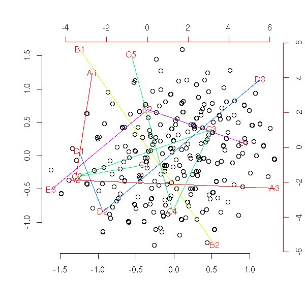
With dependant variables.
my.am(to.factor(x2))
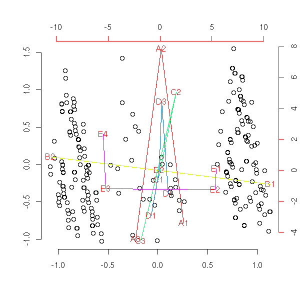
my.am(to.factor(x2, number=3))
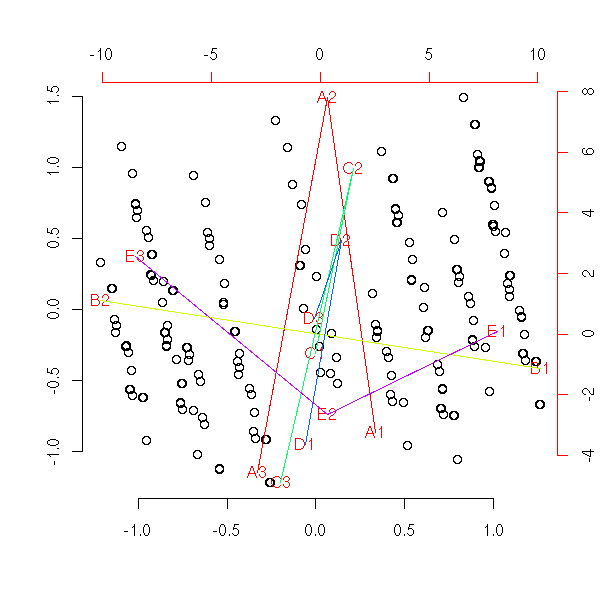
Check the "ade4" package.
The log-linear model has a role similar to that of multiple correspondance analysis -- with the added advantage that, as with any regression, we can perform tests. We start with a contingency table t_{i,j} and we try to write
log t_{i,j} = a_0 + a_1(i) + a_2(j) + a_3(i,j).This can be immediately generalized in higher dimensions (but the notations become unreadable); usually we only consider interactions of two or three variables, not more, otherwise we woud have too many parameters for the number of observations at hand.
With R, it is simply the "glm" function, with the "family=poisson" argument. .
m <- data.frame(table(random.data.1()))
y <- m[,4]
x1 <- m[,1]
x2 <- m[,2]
x3 <- m[,3]
summary(glm( y ~ x1 + x2 + x3, family=poisson ))
It yields:
> summary(glm( y ~ x1 + x2 + x3, family=poisson ))

Call:
glm(formula = y ~ x1 + x2 + x3, family = poisson)

Deviance Residuals:
    Min       1Q   Median       3Q      Max
-2.6060  -0.8723  -0.2724   0.4264   3.2634

Coefficients:
              Estimate Std. Error  z value Pr(>|z|)
(Intercept)  9.981e-01  2.965e-01    3.366 0.000762 ***
x12          3.314e-01  2.476e-01    1.338 0.180799
x13          1.643e-01  2.568e-01    0.640 0.522302
x22         -4.000e-02  1.999e-01   -0.200 0.841418
x32          5.129e-02  3.203e-01    0.160 0.872784
x33          5.057e-09  3.244e-01 1.56e-08 1.000000
x34          1.001e-01  3.163e-01    0.316 0.751674
x35          1.001e-01  3.166e-01    0.316 0.751912
---
Signif. codes:  0 `***' 0.001 `**' 0.01 `*' 0.05 `.' 0.1 ` ' 1

(Dispersion parameter for poisson family taken to be 1)

    Null deviance: 38.794  on 29  degrees of freedom
Residual deviance: 36.735  on 22  degrees of freedom
AIC: 139.11

Number of Fisher Scoring iterations: 4
TODO: understand this result
TODO: explain how to add/remove some interaction terms

> r1 <- glm( y ~ x1 + x2 + x3 + x1*x2 + x2*x3 + x1*x3, family=poisson )
> r2 <- glm( y ~ x1 + x2 + x3, family=poisson )
> anova(r1,r2)
Analysis of Deviance Table

Model 1: y ~ x1 + x2 + x3 + x1 * x2 + x2 * x3 + x1 * x3
Model 2: y ~ x1 + x2 + x3
  Resid. Df Resid. Dev  Df Deviance
1         8     6.9906
2        22    13.1344 -14  -6.1438
TODO: Introduction

TODO: This is supervised learning, it should make up a separate chapter.
We try to predict a qualitative variable, such as "has the patient just had a heart attack?", with quantitative variables, corresponding to potential risk factors (blood pressure, daily calory intake, workout, weight, etc.). We try to determine which factors are the most prevalent, i.e., which variables determine best the qualitative.
We can also use discriminant factor analysis in a predictive way, i.e., to answer the question "will the patient have a heart attack?".
TODO: explain how we do this.
More precisely, the variable to predict clusters the subjects into
several classes and we are looking for a linear combination of the
predictive variables on which we can see the separation between the
clusters.

TODO: check what follows.

I guess we try to maximize the quotient of the
mean of the variances of this linear combination in each group
and its global variance (as for anova).

???
For a binary variable:
  Normalize the predictive variables
  Compute their variance-covariance matrix A
  Compute the vector w of the means of the differences for both groups
  One can show that (?) A w = d
  w = A^-1 * d, these are the weights we were looking for

(It is a good idea to plot the observations -- in dimension higher
than two, you can use ggobi to rotate the figure.)

Diagnostics:
  Confusion matrix: rows: real values
                    columns: predicted values,
                    entries: number of cases
  From the confusion matrix, we can build more than a dozen
  different measures of the relevance of those results.
    http://149.170.199.144/multivar/da4.htm

We can first try to predict the dimension, for instance, with a
principal component analysis.

One can also perform a stepwise discriminant analysis.

library(MASS)
n <- 100
k <- 5
x1 <- runif(k,-5,5) + rnorm(k*n)
x2 <- runif(k,-5,5) + rnorm(k*n)
x3 <- runif(k,-5,5) + rnorm(k*n)
x4 <- runif(k,-5,5) + rnorm(k*n)
x5 <- runif(k,-5,5) + rnorm(k*n)
y <- factor(rep(1:5,n))
plot(lda(y~x1+x2+x3+x4+x5))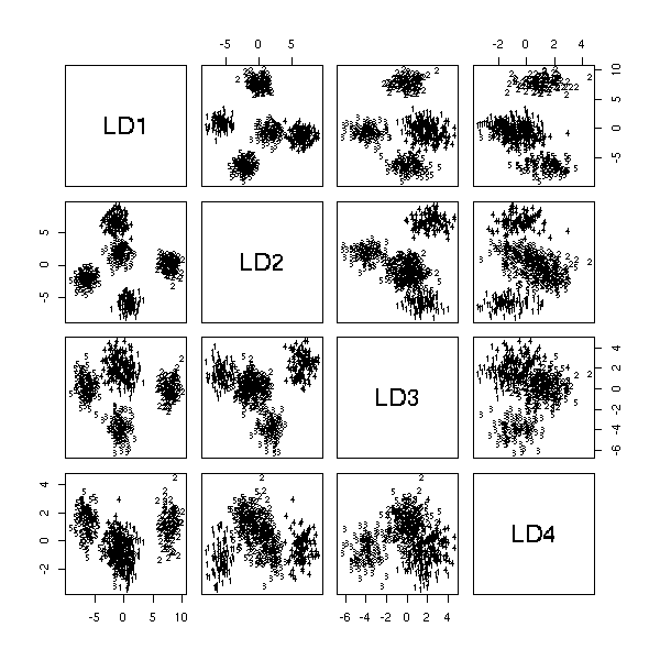
We can choose to retain only the first two dimensions.
plot(lda(y~x1+x2+x3+x4+x5), dimen=2)

Or even, just the first.
op <- par(mar=c(4,4,0,2)+.1)
plot(lda(y~x1))
par(op)
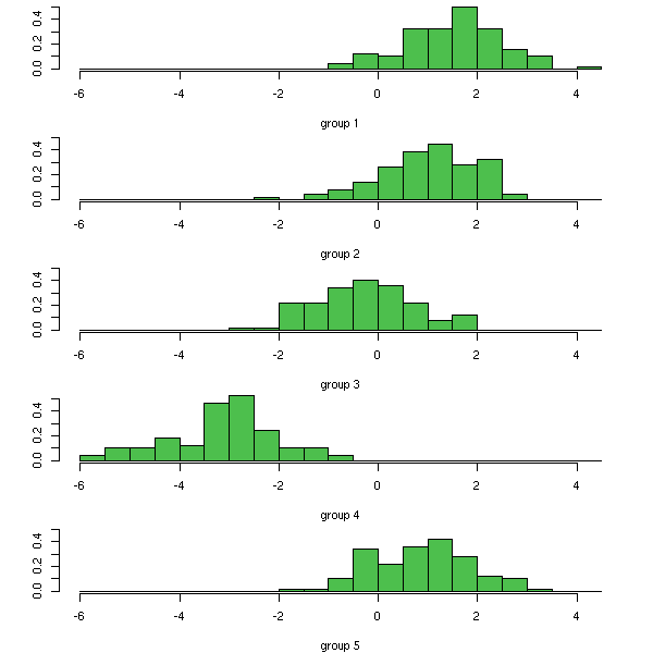
As for Principal Component Analysis, we choose the number of dimension to retain from the eigen values.
plot(lda(y~x1+x2+x3+x4+x5)$svd, type='h')
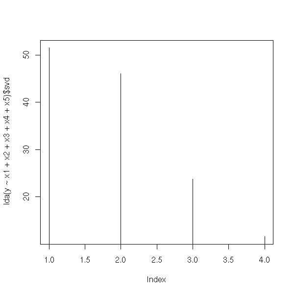
Linear discriminant analysis (LDA) can be sensitive to heteroskedasticity problems: of the two groups you are trying to separate have different variances (sizes), the boundary will be shifted to the most compact one.
The "qda" and "predict.qda" has the same role, but in a non-linear (quadratic) setting.
?qda
Also check the "mda" package.
It is the same, but we know the probabilities
P ( Y == i ),
i.e., the size of the various clusters.
(We still use the "lda" function, with one more argument.)
TODO: Example
We consider qualitative variables X1, X2, ..., Xp, Y1, Y2, ..., Yq and we look for a linear combination Xa of the Xi and a linear combination Yb of the Yj so that Xa and Yb be as correlated as possible.
library(ade4)
?cca
See for example part 4 of
http://www.cg.ensmp.fr/%7Evert/talks/021205inria/inria.pdf
Instead of using the correlation, one can use the covariance.
TODO
TODO: Explain the relations/differences between PLS and CA.
TODO: rewrite the introduction

Methods such as Principal Component Analysis (PCA) can reduce the
dimension of the cloud of points but, as they are linear, they will
not enable us to "untangle" the data: it will remain curved, it will
not become a straight segment.
One idea to straighten the curve is to embed our space (which can already be of unreasonably high dimension) into a higher-dimensional space, in a non-linear way. By applying linear methods on this higher-dimensional space, we can hope to see phenomena that were non-linear in the first space.
Here is an example of such an embedding:
(x,y) ---> (x^2, x*y, y^2).
It might sound unreasonnable to embed a space whose dimension is already problematic into an even larger one. It would indeed be the case if we needed to compute (and store) the coordinates of the points in this new space -- but actually, we only need to be able to compute scalar products.
More precisely, principal component analysis (and other similar techniques) play with the variance-covariance matrix
t(m) %*% m
In our new space, this becomes:
# Data
n <- 200  # Number of patients, number of columns
k <- 10   # Dimension of the ambient space
nb.points <- 5
p <- matrix( 5*rnorm(nb.points*k), nr=k )
library(splines)
barycentre2 <- function (y,n) {
  m <- length(y)
  x <- 1:m
  r <- interpSpline(x,y)
  #r <- lm( y ~ bs(x, knots=m) )
  predict(r, seq(1,m,length=n))$y
}
data.curve <- apply(p, 1, barycentre2, n)
data.curve <- t(data.curve)
pairs(t(data.curve))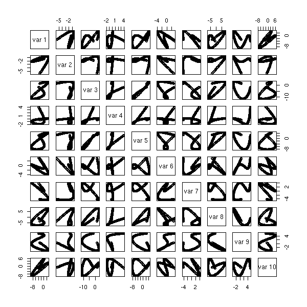
m <- data.curve
mm <- apply(m, 2, function (x) { x %o% x } )
r <- princomp(t(mm))
plot(r)
pairs(r$scores[,1:5])

Nothing exciting...
Let us try with a higher degree.
# Degree 1 kernel ("noyau" is the French word for "kernel")
noyau1 <- function (x,y) { sum(x*y) }
m <- data.curve
m <- t(t(m) - apply(m,2,mean))
k <- dim(m)[1]
wrapper <- function(x, y, my.fun, ...) {
  sapply(seq(along=x), FUN = function(i) my.fun(x[i], y[i], ...))
}
mm <- outer(1:k, 1:k, wrapper, function (i,j) { noyau1(m[,i],m[,j]) })

# Degree 2 kernel
noyau2 <- function (x,y) {
  a <- x*y
  n <- length(a)
  i <- gl(n,1,n^2)
  j <- gl(n,n,n^2)
  i <- as.numeric(i)
  j <- as.numeric(j)
  w <- which( i <= j & j <= k )
  i <- i[w]
  j <- j[w]
  sum(a[i]*a[j])
}
stopifnot( noyau2(1:2,2:1) == 12 )

# Degree 3 kernel
noyau3 <- function (x,y) {
  a <- x*y
  n <- length(a)
  i <- gl(n,1,n^3)
  j <- gl(n,n,n^3)
  k <- gl(n,n^2,n^3)
  i <- as.numeric(i)
  j <- as.numeric(j)
  k <- as.numeric(k)
  w <- which( i <= j & j <= k )
  i <- i[w]
  j <- j[w]
  k <- k[w]
  sum(a[i]*a[j]*a[k])
}
stopifnot( noyau3(1:2,2:1) == 32 )

wrapper <- function(x, y, my.fun, ...) {
  sapply(seq(along=x), FUN = function(i) my.fun(x[i], y[i], ...))
}
k <- dim(m)[1]
mm <- outer(1:k, 1:k, FUN=wrapper, my.fun = function (i,j) { noyau3(m[,i],m[,j]) })

r <- princomp(covmat=mm)
plot(r)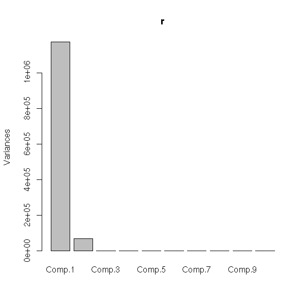
#pairs(r$scores[,1:5])
plot((t(m) %*% r$loadings) [,1:2])
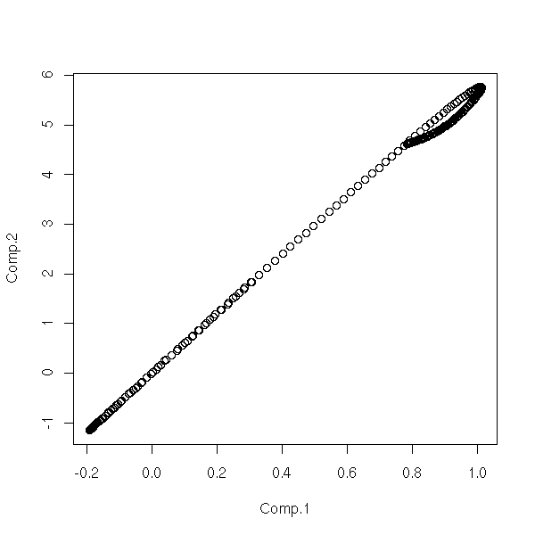
data.noisy.curve <- data.curve + rnorm(length(data.curve))
k <- dim(data.noisy.curve)[1]
mm <- outer(1:k, 1:k, FUN=wrapper, my.fun = function (i,j) {
  noyau3(data.noisy.curve[,i],data.noisy.curve[,j])
})
r <- princomp(t(data.noisy.curve), covmat=mm)
plot(r)
pairs((t(m) %*% r$loadings) [,1:5])
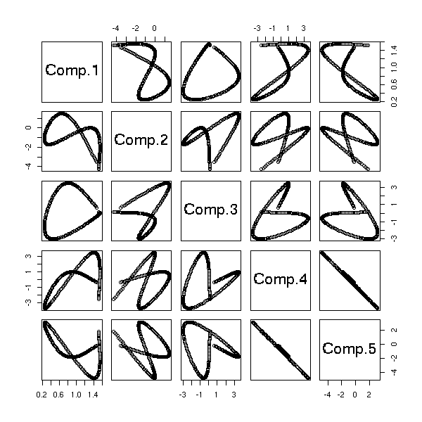
plot((t(m) %*% r$loadings) [,1:2])
lines((t(m) %*% r$loadings) [,1:2], col='red')
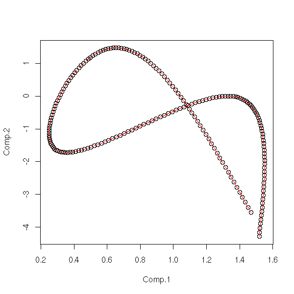
x <- 1:dim(data.noisy.curve)[2]
y1 <- (t(m) %*% r$loadings) [,1]
y2 <- (t(m) %*% r$loadings) [,2]
r1 <- loess(y1~x)
r2 <- loess(y2~x)
plot(y1,y2)
lines(y1,y2, col='red')
lines(predict(r1), predict(r2), col='blue', lwd=3)

Let us try to combine those kernels.
noyau <- function (x,y) {
  noyau1(x,y) + noyau2(x,y) + noyau3(x,y)
}
mm <- outer(1:k, 1:k, FUN=wrapper, my.fun = function (i,j) {
  noyau(data.curve[,i],data.curve[,j])
})
r <- princomp(covmat=mm)
plot(r)
pairs((t(m) %*% r$loadings) [,1:5])

Well, in the end it is not very conclusive...
Actually, there is already a package to perform those computations.
TODO: Examples
TODO...
A perceptron is a neural network with no hidden layer and binary output(s).
perceptron_learn <- function (input, output,
                              max_iterations = 100) {
  stopifnot( is.matrix(input),
             is.matrix(output),
             is.numeric(input),
             is.logical(output) )
  stopifnot( dim(input)[2] == dim(output)[2] )
  input <- rbind(input, rep(1, N)) # Biases
  N <- dim(input)[2]
  dim_input  <- dim(input)[1]
  dim_output <- dim(output)[1]
  W <- matrix(rnorm(dim_input) * rnorm(dim_output),
              nc = dim_input, nr = dim_output)
  hardlim <- function (x) ifelse( x > 0, 1, 0 )
  finished <- FALSE
  remaining_iterations <- max_iterations
  while (! finished) {
    W_previous <- W
    for (i in 1:N) {
      forecast <- hardlim( W %*% input[,i] )
      error <- output[,i] - forecast
      W <- W + error %*% input[,i]
    }
    remaining_iterations <- remaining_iterations - 1
    finished <- remaining_iterations <= 0 |
                sum(abs(W - W_previous)) < 1e-6
  }
  attr(W, "converged") <- all(W == W_previous)
  dimnames(W) <- list(output=NULL, input=NULL)
  class(W) <- "perceptron"
  W
}
perceptron_predict <- function (W, input) {
  input <- as.matrix(input)
  N <- dim(input)[2]
  input <- rbind(input, rep(1, N)) # Biases
  stopifnot( dim(W)[2] == dim(input)[1] )
  W %*% input
}

# Test
k <- 2   # BUG: It does not work with other values...
N <- 50
set.seed(1)
centers <- matrix(rnorm(2*k), nc=2)
output <- sample(1:k, N, replace=T)
input <- t(matrix(
  rnorm(k*N, mean=centers[output,], sd=.1),
           nc=2))
output <- t(output == 1)
w <- perceptron_learn(input, output)

plot(t(input), col=1+output,
     xlab="", ylab="", main="Perceptron learning")
abline(-w[3]/w[2], -w[1]/w[2], lwd=3, lty=2)
%%G
# It is not designed to work if the clusters overlap:
# It will fail to converge...
N <- 50
set.seed(2)
centers <- matrix(rnorm(2*k), nc=2)
output <- sample(1:k, N, replace=T)
input <- t(matrix(
  rnorm(k*N, mean=centers[output,], sd=1),
           nc=2))
output <- t(output == 1)
w <- perceptron_learn(input, output)

plot(t(input), col = 1 + output,
     xlab = "", ylab = "",
     main = "Perceptron failing to converge")
abline(-w[3]/w[2], -w[1]/w[2], lwd=3, lty=2)
%--

library(MASS)
z <- output[1,]
x <- input[1,]
y <- input[2,]
r <- lda( z ~ x + y )
n <- 200
x <- rep(seq(-2,2,length=n), each=n)
y <- rep(seq(-2,2,length=n), n)
z <- predict(r, data.frame(x, y))
z <- c(rgb(.7,.7,.7), rgb(1,.7,.7))[ as.numeric(z$class) ]
plot(x, y, col=z, pch=15,
     xlab="", ylab="",
     main="Non-converging perceptron and LDA")
points(t(input), col = 1 + output)
abline(-w[3]/w[2], -w[1]/w[2], lwd=3, lty=2)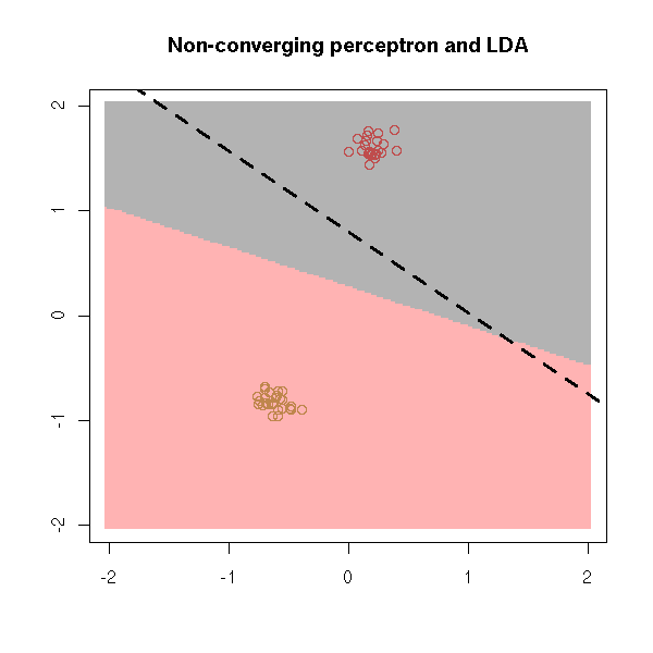
library(e1071)
y <- as.factor(output[1,])
x <- t(input)
r <- svm(x, y)
n <- 200
x <- cbind( rep(seq(-2,2,length=n), each=n),
            rep(seq(-2,2,length=n), n)       )
z <- predict(r, x)
z <- c(rgb(.7,.7,.7), rgb(1,.7,.7))[ as.numeric(z) ]
plot(x, col=z, pch=15,
     xlab="", ylab="",
     main="Non-converging perceptron and SVM")
points(t(input), col = 1 + output)
abline(-w[3]/w[2], -w[1]/w[2], lwd=3, lty=2)
Perceptrons should not be used if the cloud of points is not separable: in this case, prefer logistic regression, linear discriminant analysis (LDA) or support vector machines (SVM).
TODO
In the statistical community, this is known as "(least
squares) linear regression".
Windrow-Hoff learning rule: gradient descent for linear
filter neurons -- i.e., for least squares linear
regression.

Back-propagation: gradient descent algorithm for
multi-layer networks.
The tricky point is to compute the gradient (there are too
many variables to do this by applying a general method):
this is what the back-propagation algorithm provides.

Feed-forward neural network: this is the classical 3-layer
(i.e., with one hidden layer) neural net, fitted by
back-propagation.

Batch training: for each update of the weights, you use
all the data.
Incremental training, on-line learning: you only use one
observation to update the weights.

Variants of gradient descent:

  Gradient descent with momentum (this increases the
  convergence speed; it is not too dissimilar to tabu
  search).

  Variable learning rate: if the previous move did not
  decrease the error, i.e., if we went too far in the
  direction of the gradient, decrease the learning rate by
  30%, if not, increase it by 5%.

  Resilient back-propagation (Rprop): since sigmoid
  function tend to squash their inputs, even very wrong
  weights can induce a small change in the result -- this
  leads to a very slow convergence toward the optimal
  weights.  Resilient back-propagation only uses the sign
  of the derivative. The amplitude of the change is
  controled by another parameter that increases if there
  have been two successive changes in the same direction
  and decreases if there have been two successive changes
  in opposite directions.

  Conjugate gradient:
  Look in the direction of the (opposite of the) gradient
  and perform a line search in this direction.
  The next direction is not the opposite of the gradient
  but a linear combination of the opposite of the gradient
  and the previous search direction.
    new direction = - gradient + beta * old direction
  where (Fletcher-Reeves update)
            norm(current gradient) ^ 2
    beta = -----------------------------
            norm(previous gradient) ^ 2
  or (Polak-Ribiere update)
            < current gradient - previous, current >
    beta = -------------------------------------------
                 norm( previous gradient ) ^ 2
  From time to time (e.g., after as many iterations as
  there are parameters, or when the angle between two
  successive gradients becomes too high (Powel_Beale
  restarts)), reset the direction to the opposite of the
  gradient.

  Quasi-newton: The newton method is very fast, but it
  requires second derivatives (hessian matrices), which
  are too expensive to compute for neural networks.
  Quasi-newton algorithms try to approximate it without
  the second derivative computational overhead.

  BFGS quasi-Newton algorithm: an approximation of the
  hessian matrix is stored and updated at each iteration,
  using the gradient. (details?)

  One-step secant quasi-Newton algorithm: idem, but
  assumes that the previous estimation of the hessian was
  the identity matrix -- hence, there is no need to store
  it.

  Levenberg-Maquardt: This is yet another quasi-Newton
  method.s
    x[k+1] = x[k] - (J' + mu I)^-1 J' error
  where
    x: parameters to be estimated
    J = d error / d weights
    gradient = J' error
    hessian = J' J (approximately)
    mu = 0:  this is Newton's method, with an approximate
             hessian
    mu >> 0: this is a gradient method with a small step
             size

  Reduced-memory Levenberg-Maquardt: the matrix J is huge
  (its number of rows is the number of training sets). If
  ot does not fit in memory, you can cut it into blocks.10

Line search routines (for conjugate gradient methods):
  Quadratic interpolation
  Golden section search
  Brent's search (hydrid of qquadratic interpolation and
    the golden section search)
  Hybrid bisection-cubic search
  Charalambous search
  Backtracking search

Avoiding overfitting:
  Stop the algorithm when the performance on a validation
  sample starts to decrease (it may sound reasonable, but
  this is apprtoximately a baysian fit with the initial
  (random) weights as a prior...). And you must be careful
  not to choose too fast an algorithm...
  Choose a network small enough
  Add a penalty (the sum of the squares of the weights) to
  the objective function, to shrink the weights towards
  zero (try to have inputs, outputs and weights of the
  same order of magnitude, say in [-1,1]).
    Objective = lambda * Mean Square Error +
                (1 - lambda) * Mean Square Weight
You can reduce the dimension of a cloud of points with a 5-layer neural network: an input layer (with the data), a (non-linear) compression layer, a (linear) layer representing the data in the low-dimensional space, a (non-linear) uncompression layer, and an output layer (on which we expect to get the initial data back).
I do not think that such networks are already implemented in R, so we shall do it ourselves -- we shall be EXTREMELY careful with convergence problems.
As I do not really know neural networks (I was superficially interested in the subject 10 years ago), I browse the net to understand them
http://www.willamette.edu/%7Egorr/classes/cs449/backprop.html
and I write the following code.
TODO: start with a smaller example, on which the computations will
be faster and for which we know waht kind of result we should
expect. For instance, a 2-dimensional cloud in a 3-dimensional
space. with only linear neurons and only two neurons in the middle
layer.

Problem: in this case, the intermediary layers are useless and
may unstabilize the algorithm.


# x: matrix whose columns are the vectors to learn
# n: number of neurons in the middle layer
# m: number of neurons in the two other hidden layers
#     (you should have m>n)
drnn <- function (M, n, m, e=.1, N=100) {
  # Activation fucntions
  id <- function (t) { t }
  f1 <- tanh
  f2 <- id
  f3 <- tanh
  f4 <- id
  # Number of neurons in each layer
  n0 <- dim(M)[1]
  n1 <- m
  n2 <- n
  n3 <- m
  n4 <- n0
  # The weights -- initialized by random values
  w1 <- matrix( rnorm(n0*n1), nc=n0, nr=n1 )
  w2 <- matrix( rnorm(n1*n2), nc=n1, nr=n2 )
  w3 <- matrix( rnorm(n2*n3), nc=n2, nr=n3 )
  w4 <- matrix( rnorm(n3*n4), nc=n3, nr=n4 )
  # Les biais
  b1 <- rnorm(n1)
  b2 <- rnorm(n2)
  b3 <- rnorm(n3)
  b4 <- rnorm(n4)
  # The algorithm (backpropagation)
  r <- list()
  err <- rep(0, N)
  for (i in 1:N) {
    cat(paste("Iteration", i, "\n"))
    res <- matrix(NA, nr=n, nc=dim(M)[2])
    for (j in 1:dim(M)[2]) {
      x <- M[,j]
      # Computing the valu of the nodes
      y0 <- x
      y1 <- f1( w1 %*% y0 + b1 )
      y2 <- f2( w2 %*% y1 + b2 )
      y3 <- f3( w3 %*% y2 + b3 )
      y4 <- f4( w4 %*% y3 + b4 )
      # Computing the errors
      d4 <- x - y4
      d3 <- (t(w4) %*% d4) * (1 - y3^2)
      d2 <- (t(w3) %*% d3) * 1
      d1 <- (t(w2) %*% d2) * (1 - y1^2)
      # Updating the weights and the biases
      dw4 <- d4 %*% t(y3)
      dw3 <- d3 %*% t(y2)
      dw2 <- d2 %*% t(y1)
      dw1 <- d1 %*% t(y0)
      w4 <- w4 + e * dw4
      w3 <- w3 + e * dw3
      w2 <- w2 + e * dw2
      w1 <- w1 + e * dw1
      b4 <- b4 + e * d4
      b3 <- b3 + e * d3
      b2 <- b2 + e * d2
      b1 <- b1 + e * d1
      res[,j] <- y2
      err[i] <- err[i] + sum(d4^2)
    }
    r[[i]] <- res
  }
  list(scores=res, errors=err, r=r)
}

r <- drnn(data.curve, 1, 4, N=30, e=.02)
plot(r$err, ylim=range(c(0,r$err)), type='l')
%--

i <- order(drop(r$scores))
plot(t(data.curve)[,1:2])
lines(t(data.curve)[,1:2][i,], col='red')
%--
Well, it is not exactly what we were expecting. But it is still better than nothing...
op <- par(mfrow=c(2,2))
for (k in c(1, 3, 7, 30)) {
  i <- order(drop(r$r[[k]]))
  plot(t(data.curve)[,1:2], main=paste("after",k,"iteration(s)"))
  lines(t(data.curve)[,1:2][i,], col='red')
}
par(op)
%--
Changing the order in which we give the points to the network has no significant effect.
op <- par(mfrow=c(2,4))
for (i in 1:4) {
  m <- data.curve[,sample(1:dim(data.curve)[2])]
  r <- drnn(m, 1, 4, N=30, e=.02)
  plot(r$err, ylim=range(c(0,r$err)), type='l')
  i <- order(drop(r$scores))
  plot(t(m)[,1:2])
  lines(t(m)[,1:2][i,], col='red')
}
par(op)
%--
The plot of the error is VERY worrying: the error is supposed to decrease at each iteration -- it sometimes increases. Do not use this code unless you really understand it and think it is correct.
Let us try with two neurons in the middle layer.
i <- sample(1:dim(data.curve)[2])
m <- data.curve[,i]
r <- drnn(m, 2, 8, N=30, e=.02)
plot(r$err, ylim=range(c(0,r$err)), type='l')
plot(t(r$scores)[i,], type='l')
%--
(Yes, it is supposed to be a curve...)
TODO: look more precisely what happens when we change one of the
parameters. Each time, display at least 4 plots: the error (that
should be decreasing), the first path, the last path.

TODO: Check that my implementation is correct.
The evolution of the error term suggest there IS a problem.
Neural networks can help increase the coverage and the precision of OS fingerprinting (this could apply to any rules-based classifier):
http://actes.sstic.org/SSTIC06/Fingerprinting_par_reseaux_neuronaux/
0. Data
1. Kernels
2. Neural networks
3. k-means + MST
4. Isomap
5. Optimisation
6. pruned MST
7. TSP
8. SVM
Let us consider a cloud of (40) points in a space of reasonable dimension (10) or of less reasonable dimension (7000). The points are more or less aligned on a curve we are trying to describe.
The real situation was the following. With DNA array, we examined the expression of 7000 genes in 40 patients, representing different stages of a single disease. We can see this pattern by a Principal Component Analysis (PCA) (or via other dimension reduction techniques): the points give the impression of forming a curve. In dimension two, the curve may seem singular, it seem to cross itself, but in higher dimension, it looks smooth. With the expression of those genes (all of them or, rather, just a subset of them), we would like to define an "index" indicating the position on the curve and, thus, the current stage of the disease.
We shall first describe the data (both simulated data and real data), apply various classical dimension reduction techniques (PCA, PCA after non-linear transformations, neural networks), some less classical ones (based on optimization problems such as the traveling salesman problem) and we shall compare all those methods.
Simulated data: broken line.
n <- 200  # Number of patients, number of columns
k <- 10   # Dimension of the ambient space
nb.points <- 5
p <- matrix( 5*rnorm(nb.points*k), nr=k )
barycentre <- function (x, n) {
  # Add number between the values of x in order to get a length n vector
  i <- seq(1,length(x)-.001,length=n)
  j <- floor(i)
  l <- i-j
  (1-l)*x[j] + l*x[j+1]
}
m <- apply(p, 1, barycentre, n)
data.broken.line <- t(m)
pairs(t(data.broken.line))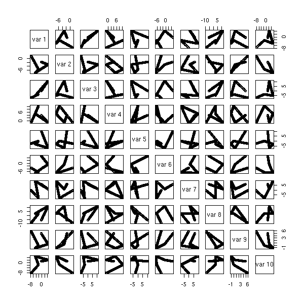
plot(princomp(t(data.broken.line)))

pairs(princomp(t(data.broken.line))$scores[,1:5])
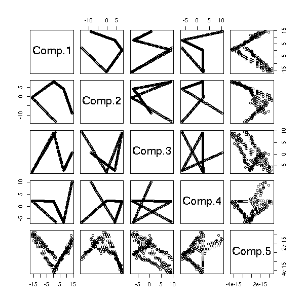
Simulated data: noisy broken line
data.noisy.broken.line <- data.broken.line + rnorm(length(data.broken.line))
pairs(princomp(t(data.noisy.broken.line))$scores[,1:5])

Simulated data: curve -- we just change our "barycentre" function.
library(splines)
barycentre2 <- function (y,n) {
  m <- length(y)
  x <- 1:m
  r <- interpSpline(x,y)
  #r <- lm( y ~ bs(x, knots=m) )
  predict(r, seq(1,m,length=n))$y
}

k <- 5
y <- sample(1:100,k)
x <- seq(1,k,length=100)
plot(barycentre2(y,100) ~ x)
lines(y, col='red', lwd=3, lty=2)
data.curve <- apply(p, 1, barycentre2, n)
data.curve <- t(data.curve)
pairs(t(data.curve))
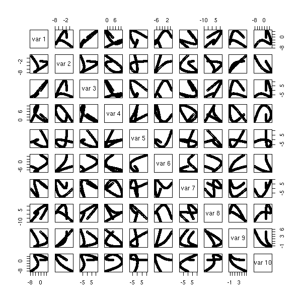
plot(princomp(t(data.curve)))
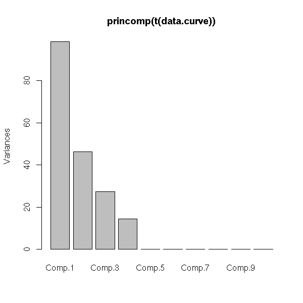
pairs(princomp(t(data.curve))$scores[,1:5])
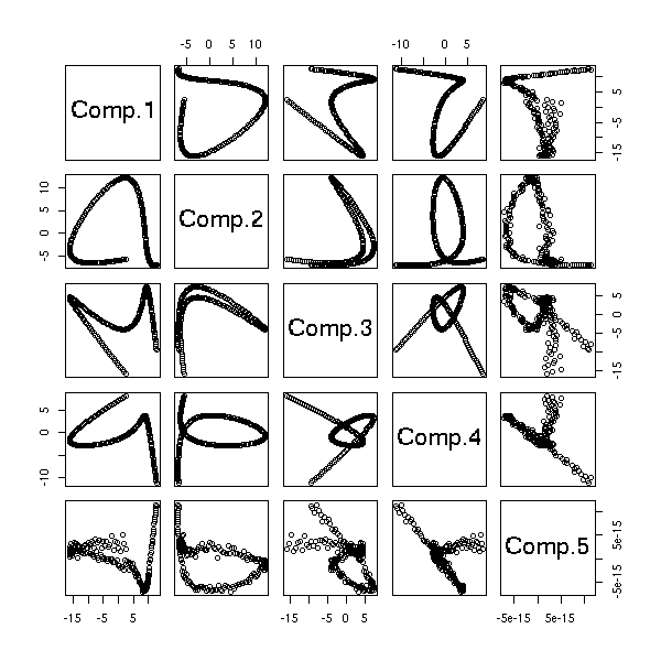
Some more noise:
data.noisy.curve <- data.curve + rnorm(length(data.curve))
pairs(t(data.noisy.curve))

plot(princomp(t(data.noisy.curve)))

pairs(princomp(t(data.noisy.curve))$scores[,1:5])
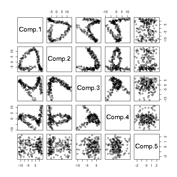
Let us think about the shape of the curve we would expect. If the disease is lethal (or if, for all the patients of the study, it evolves towards death), we can expect a segment, curved, one end representing healthy people, the other dead patients.
If the disease is benign, we would expect the points to form a (deformed) circle, representing the successives stages of the disease, until a once-again healthy patient.
If the disease is sometimes lethal, sometimes not, we could expect a mixture of both: the reunion of a circle and a segment.
random.rotation.matrix <- function (n=3) {
  m <- NULL
  for (i in 1:n) {
    x <- rnorm(n)
    x <- x / sqrt(sum(x*x))
    y <- rep(0,n)
    if (i>1) for (j in 1:(i-1)) {
      y <- y + sum( x * m[,j] ) * m[,j]
    }
    x <- x - y
    x <- x / sqrt(sum(x*x))
    m <- cbind(m, x)
  }
  m
}

n <- 200
k <- 10
x <- seq(0,2*pi,length=n)
data.circle <- matrix(0, nr=n, nc=k)
data.circle[,1] <- cos(x)
data.circle[,2] <- sin(x)
data.circle <- data.circle %*% random.rotation.matrix(k)
data.circle <- t( t(data.circle) + rnorm(k) )
pairs(data.circle[,1:3])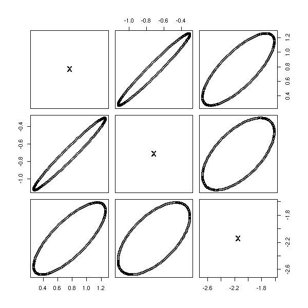
data.circle <- data.circle + .1*rnorm(n*k)
pairs(data.circle[,1:3])
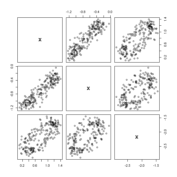
pairs(princomp(data.circle)$scores[,1:3])

TODO: The other example
Real data:
data.real <- read.table("Tla_z.txt", sep=",")
data.real.group <- factor(substr(names(data.real),0,1))
r <- prcomp(t(data.real))
plot(r$sdev, type='h')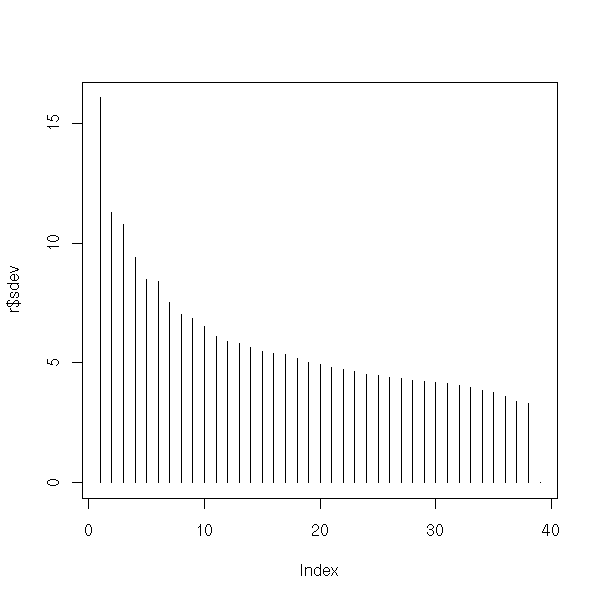
data.real.3d <- r$x[,1:3]
pairs(data.real.3d, pch=16, col=as.numeric(data.real.group))

To see more clearly what happens, let us add an ellipse for each group of points.
draw.ellipse <- function (
    x, y=NULL, N=100,
    method=lines, ...
  ) {
  if (is.null(y)) {
    y <- x[,2]
    x <- x[,1]
  }
  centre <- c(mean(x), mean(y))
  m <- matrix(c(var(x),cov(x,y),
                cov(x,y),var(y)),
              nr=2,nc=2)
  e <- eigen(m)
  r <- sqrt(e$values)
  v <- e$vectors
  theta <- seq(0,2*pi, length=N)
  x <- centre[1] + r[1]*v[1,1]*cos(theta) +
       r[2]*v[1,2]*sin(theta)
  y <- centre[2] + r[1]*v[2,1]*cos(theta) +
       r[2]*v[2,2]*sin(theta)
  method(x,y,...)
}
draw.star <- function (x, y=NULL, ...) {
  if (is.null(y)) {
    y <- x[,2]
    x <- x[,1]
  }
  d <- cbind(x,y)
  m <- apply(d, 2, mean)
  segments(m[1],m[2],x,y,...)
}
my.plot <- function (
    d, f=rep(1,dim(d)[1]),
    col=rainbow(length(levels(f))),
    variables=NULL, legend=T, legend.position=1,
    draw=draw.ellipse, ...) {
  xlim <- range(d[,1])
  ylim <- range(d[,2])
  if(!is.null(variables)){
    xlim <- range(xlim, variables[,1])
    ylim <- range(ylim, variables[,2])
  }
  plot(d, col=col[as.numeric(f)], pch=16,
       xlim=xlim, ylim=ylim, ...)
  for (i in 1:length(levels(f))) {
    try(
      draw(d[ as.numeric(f)==i, ], col=col[i])
    )
  }
  if(!is.null(variables)){
    arrows(0,0,variables[,1],variables[,2])
    text(1.05*variables,rownames(variables))
  }
  abline(h=0,lty=3)
  abline(v=0,lty=3)
  if(legend) {
    if(legend.position==1) {
      l=c( par('usr')[1],par('usr')[4], 0, 1 )
    } else if (legend.position==2) {
      l=c( par('usr')[2],par('usr')[4], 1, 1 )
    } else if (legend.position==3) {
      l=c( par('usr')[1],par('usr')[3], 0, 0 )
    } else if (legend.position==4) {
      l=c( par('usr')[2],par('usr')[3], 1, 0 )
    } else {
      l=c( mean(par('usr')[1:2]),
           mean(par('usr')[1:2]), .5, .5 )
    }
    legend(l[1], l[2], xjust=l[3], yjust=l[4],
           levels(f),
           col=col,
           lty=1,lwd=3)
  }
}
my.plot(data.real.3d[,1:2], data.real.group)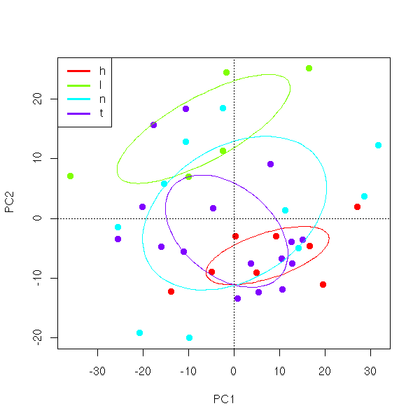
op <- par(mfrow=c(3,3), mar=.1+c(0,0,0,0))
plot.new();
my.plot(data.real.3d[,c(2,1)], data.real.group,
        xlab='',ylab='',axes=F,legend=F)
box()
my.plot(data.real.3d[,c(3,1)], data.real.group,
        xlab='',ylab='',axes=F,legend=F)
box()

my.plot(data.real.3d[,c(1,2)], data.real.group,
        draw=draw.star,
        xlab='',ylab='',axes=F,legend=F)
box()
plot.new()
my.plot(data.real.3d[,c(3,2)], data.real.group,
        xlab='',ylab='',axes=F,legend=F)
box()

my.plot(data.real.3d[,c(1,2)], data.real.group,
        draw=draw.star,
        xlab='',ylab='',axes=F,legend=F)
box()
my.plot(data.real.3d[,c(2,3)], data.real.group,
        draw=draw.star,
        xlab='',ylab='',axes=F,legend=F)
box()
plot.new()
par(op)
You can also turn the plot to see it from various angles.
set.seed(66327)
random.rotation.matrix <- function (n=3) {
  m <- NULL
  for (i in 1:n) {
    x <- rnorm(n)
    x <- x / sqrt(sum(x*x))
    y <- rep(0,n)
    if (i>1) for (j in 1:(i-1)) {
      y <- y + sum( x * m[,j] ) * m[,j]
    }
    x <- x - y
    x <- x / sqrt(sum(x*x))
    m <- cbind(m, x)
  }
  m
}
op <- par(mfrow=c(3,3), mar=.1+c(0,0,0,0))
for (i in 1:9) {
  #plot( (data.real.3d %*% random.rotation.matrix(3))[,1:2],
  #      pch=16, col=as.numeric(data.real.group),
  #      xlab='', ylab='', axes=F )
  my.plot((data.real.3d %*% random.rotation.matrix(3))[,1:2],
          data.real.group,
          draw=draw.ellipse,
          xlab='',ylab='',axes=F,legend=F)
  box()
}
par(op)
Some time ago, I have seen an article about dimension reduction (in
Rnews, or a vignette). Read it.

Implement Isomap
(easy: use MST)

Other articles
google: dimensionality reduction
We can formulate our problem as an optimization problem: we are looking for the coordinates of 5 points A1, A2, A3, A4, A5 in order to minimize the sum of the (squares of the) distances of the points in the cloud to the broken line A1-A2-A3-A4-A5.
TODO: To check that this algorithm, first give it:
- a single segment to find, in dimension 1
- a single segment to find, in dimension 2
- a curve (a flat parabola) with 1 segment
- a curve (parabola) with two segments
- only then our data.


distance.broken.line <- function (point, ligne) {
  # point: vector containing the coordinates of the point (from the
           cloud) whose distance to the broken line is to be computed.
  # ligne: coordinates, in columns, of the points defining the broken line.

  # Distance to the vertices of the broken line
  d.points <- apply( (ligne-point)^2, 2, sum )

  # Position of the projection of the point on each of the segments
  # of the broken line
  v <- t(apply(ligne,1,diff))   # Vectors  A(i)A(i+1)
  w <- -ligne + point           # Vectors  A(i)M
  w <- w[, -dim(w)[2]]          # Remove the last
  lambda <- apply(v*w, 2, sum) / apply(v^2,2,sum)
  lambda[ is.nan(lambda) ] <- 0

  # Distance to the segments of the broken line
  d.segments <- apply( (w - t(lambda*t(v)))^2, 2, sum )
  d.segments <- d.segments[ lambda>0 & lambda<1 ]

  min(c( d.points, d.segments ))
}

# Tests: the following distances ar close to zero
stopifnot( distance.broken.line(p[,1], p) < 1e-6 )
stopifnot( distance.broken.line(.5*p[,1]+.5*p[,2], p) < 1e-6 )
# There is a BIG speed problem: in the following example, we need
# two seconds to compute the distance...
sum(apply(data.noisy.broken.line, 2, distance.broken.line, p))

broken.line <- function (
    d,    # data
    np=4, # Number of segments in the broken line
    deb = as.vector(d[,sample(1:dim(d)[2], np)])
            # starting values: broken line through np poins of the cloud, at random.
  ) {
  f <- function (x) {
    sum(apply(d, 2, distance.broken.line, matrix(x, nc=np) ))
  }
  # Very, very long...
  r <- optim(deb, f, control=list(trace=1, maxit=50)) # Default: 500 iterations
  list(par=r$par, method="optim", value=r$value, deb=deb, np=np, r=r)
}

r <- broken.line(data.noisy.broken.line)
pc <- princomp(t(data.noisy.broken.line))
plot(pc$scores[,1:2])

lines( (t(matrix(r$deb,nc=r$np) - pc$center) %*% pc$loadings)[,1:2], col='red',lwd=3,lty=3)
lines((t(matrix(r$par,nc=r$np) - pc$center) %*% pc$loadings)[,1:2], col='blue',lwd=3,lty=2)
%--


# Example: a segment, in dimension 1
l <- c(-5, 3, 2, -1)
deb <- c(1,2,3,4)
d <- rbind( seq(l[1],l[2],length=10), seq(l[3],l[4],length=10) )
r <- broken.line(d, np=2, deb=deb)
plot(t(d), xlim=c(-10,10), ylim=c(-10,10))
# Be careful about the order of the parameters to estimate...
for (i in 1:100) { lines(matrix(sample(r$par), nr=2) ) }
%--


# Starting values: some points of the cloud, at random
op <- par(mfrow=c(3,3), mar=.1+c(0,0,0,0))
for (i in 1:9) {
  l <- runif(4, -8,8)
  d <- rbind( seq(l[1],l[2],length=10), seq(l[3],l[4],length=10) )
  r <- broken.line(d, np=2)
  plot(t(d), xlim=c(-10,10), ylim=c(-10,10),
       xlab='', ylab='', axes=F)
  box()
  lines( r$par[c(1,3)], r$par[c(2,4)], col='red' )
}
par(op)
%--

# Starting values: random
op <- par(mfrow=c(3,3), mar=.1+c(0,0,0,0))
for (i in 1:9) {
  l <- runif(4, -8,8)
  deb <- runif(4, -8,8)
  d <- rbind( seq(l[1],l[2],length=10), seq(l[3],l[4],length=10) )
  r <- broken.line(d, np=2, deb=deb)
  plot(t(d), xlim=c(-10,10), ylim=c(-10,10),
       xlab='', ylab='', axes=F)
  box()
  lines( r$par[c(1,3)], r$par[c(2,4)], col='red' )
  lines( deb[c(1,3)], deb[c(2,4)], col='blue', lty=2 )
}
par(op)
%--
Aaaaaaahhhhhhhhhhhh... It does not converge -- not at all. Let us try again, by running the algorithm several times.
op <- par(mfrow=c(3,3), mar=.1+c(0,0,0,0))
for (i in 1:9) {
  l <- runif(4, -8,8)
  deb <- runif(4, -8,8)
  d <- rbind( seq(l[1],l[2],length=10), seq(l[3],l[4],length=10) )
  plot(t(d), xlim=c(-10,10), ylim=c(-10,10),
       xlab='', ylab='', axes=F)
  box()
  lines( deb[c(1,3)], deb[c(2,4)], col='blue', lty=2 )
  for (j in 1:10) {
    r <- broken.line(d, np=2, deb=deb)
    lines( r$par[c(1,3)], r$par[c(2,4)], col='red' )
    deb <- r$par
  }
}
par(op)
%--
No, it really fails to converge.
TODO: look at the value of the distance at the end of the
algorithm...
I get very small values while the segment id rather far away from
the points: why?
(this bug could account for the convergence problems...)
There is another problem: the solution we are looking for is not unique. If a segment is a solution of our problem, any larger segment is also a solution.
It converges too slowly to get a reliable result. Let us try ith the nlm function ("optim" should work fine with "naughty" functions, "nlm" on "nice" functions -- our function os piecewise quadratic, with a unique local minimum).
# Even longer...
r <- nlm(f, deb, iterlim=20)   # By default, iterlim=100...
pc <- princomp(t(data.noisy.broken.line))
plot(pc$scores[,1:2])
lines( (t(matrix(deb, nc=np) - pc$center) %*% pc$loadings)[,1:2], col='red', lwd=3, lty=3 )
lines((t(matrix(r$estimate,nc=np) - pc$center) %*% pc$loadings)[,1:2], col='blue', lwd=3, lty=2)
In the previous example (had it worked), the curve was made of 4 segments and we wer looking for a curve made of 3 segments. If we had asked for 5 segments, we would have had a segment of length 0, or an unused segment at the end of the curve. to avoid this, we can add a penalty if the segments do not have the same length.
# I add the sum of the inverses of the squares of the lengths of the
# segments.
# TODO: This is a BAD idea: it favours long, useless segments.
f <- function (x) {
  sum(apply(data.noisy.broken.line, 2, distance, matrix(x, nc=np) )) +
  sum( 1/apply(t(apply(matrix(x,nc=np), 1,diff))^2, 2, sum) )
}

TODO: computation with 6 or 7 segments to find a broken line with
only 5.

TODO: Similarly, we could add a penalty for the total length of the
curve.

TODO: We could do the same thing with splines
The Traveling Salesman Problem is the following: we have a cloud of points (in a metric space: think "cities on a map") and we are looking for a path, as short as possible, that visits each point. On other words, we want to find an order on the points that minimizes a certain function.
Presented like that, the problem already has a lot of applications (for instance, the path of a delivery car; the path of a soldering iron in an electrnic appliances assembly line), but other seemingly unrelated problems can be formulated as TSP (for instance, some problems in gene mapping -- see Setubal's book -- I confess I have never read it).
We can apply a TSP-solving algorithm to our cloud of points: we get an order on those points, that can be seen as a broken line. We then smooth this broken line: we get a curve, parametrized by [0,1] -- this parameter is the index we were looking for. Finally, given a new point, we just have to project it onto the curve to get the value of the parameter.
Unfortunately, no TSP-solving algorithm is implemented under R: we shall have to program.
Here is an implementation using descent: we start with a random path (i.e., an order on the points) and we try to transform it (by interchanging the rank of two points) to get a shorter path.
longueur <- function (d,o) {
  n <- length(o)
  sum(diag( d [o[1:(n-1)],] [,o[2:n]] ))
}
tsp.descent <- function (d, N=1000) {
  # d: distance matrix
  d <- as.matrix(d)
  n <- dim(d)[1]
  o <- sample(1:n)
  v <- longueur(d,o)
  k <- 0
  res <- list()
  k.res <- c()
  l.res <- c(v)
  while (k<N) {
    i <- sample(1:n, 2)
    oo <- o
    oo[ i[1] ] <- o[ i[2] ]
    oo[ i[2] ] <- o[ i[1] ]
    w <- longueur(d,oo)
    if (w<v) {
      v <- w
      o <- oo
      res <- append(res, list(o))
      k.res <- append(k.res, k)
      l.res <- append(l.res, v)
      k <- 0
    } else {
      k <- k+1
    }
  }
  list(o=o, details=res, k=k.res, longueur=v, longueurs=l.res)
}

n <- 100
x <- matrix(runif(2*n), nr=n)
r <- tsp.descent(dist(x))
o <- r$o
plot(x)
lines(x[o,], col='red')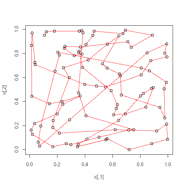
op <- par(mfrow=c(2,2))
n <- length(r$details)
for (i in floor(c(1, n/4, n/2, n))) {
  plot(x, main=paste("n =",i))
  lines(x[r$details[[i]],], col='red')
}
par(op)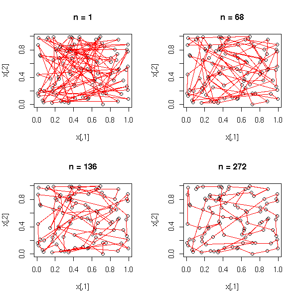
The value we have chosen for N is not sufficient:
plot(r$k)
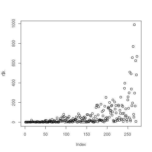
n <- 100
x <- seq(0,6, length=n)
x <- sample(x)
x <- cbind(cos(x), sin(x))
r <- tsp.descent(dist(x), N=10000)
op <- par(mfrow=c(2,2))
n <- length(r$details)
for (i in floor(c(1, n/4, n/2, n))) {
  plot(x, main=paste("n =",i))
  lines(x[r$details[[i]],], col='red')
}
par(op)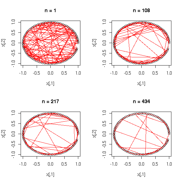
plot(r$k)
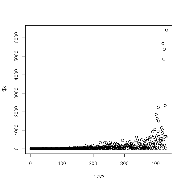
We can try to improve the algorithm by running it several times.
# Very long...
op <- par(mfrow=c(3,3))
for (i in 1:9) {
  r <- tsp.descent(dist(x), N=1000)
  plot(x, main=signif(r$longueur))
  lines( x[r$o,], col='red', type='l' )
}
par(op)
Still not conclusive.
We can modify the algorithm above by accepting a new path even if it is worse, with a probability initially high, but that progressively decreases.
tsp.recuit <- function (d, N=1000, taux=.99) {
  # d: distance matrix
  d <- as.matrix(d)
  n <- dim(d)[1]
  o <- sample(1:n)
  v <- longueur(d,o)
  # Computing the initial temperature
  dE <- NULL
  j <- 0
  for (i in 1:100) {
    i <- sample(1:n, 2)
    oo <- o
    oo[ i[1] ] <- o[ i[2] ]
    oo[ i[2] ] <- o[ i[1] ]
    w <- longueur(d,oo)
    if (w<v) {
      dE <- append(dE,abs(w-v))
      j <- j+1
    }
  }
  print(dE)
  T <- - max(dE) / log(.8)
  print(T)
  # Initialisations
  k <- 0
  res <- list()
  k.res <- c()
  l.res <- c(v)
  t.res <- c(T)
  p.res <- c()
  while (k<N) {
    i <- sample(1:n, 2)
    oo <- o
    oo[ i[1] ] <- o[ i[2] ]
    oo[ i[2] ] <- o[ i[1] ]
    w <- longueur(d,oo)
    p.res <- append(p.res, exp((v-w)/T))
    if ( runif(1) < exp((v-w)/T) ) {
      v <- w
      o <- oo
      res <- append(res, list(o))
      k.res <- append(k.res, k)
      l.res <- append(l.res, v)
      k <- 0
      T <- T*taux
      t.res <- append(t.res, T)
    } else {
      k <- k+1
    }
  }
  list(o=o, details=res, k=k.res, longueur=v, longueurs=l.res, T=t.res, p=p.res)
}

n <- 100
x <- seq(0,5, length=n)
x <- sample(x)
x <- cbind(cos(x), sin(x))
r <- tsp.recuit(dist(x), N=1000, taux=.995)
op <- par(mfrow=c(2,2))
n <- length(r$details)
for (i in floor(c(1, n/4, n/2, n))) {
  plot(x, main=paste("n =",i))
  lines(x[r$details[[i]],], col='red')
}
par(op)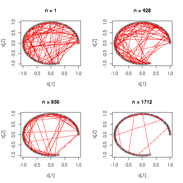
op <- par(mfrow=c(2,2))
plot(r$k)
plot(r$longueurs, main="Lengths")
plot(r$T, main="Temperature")
plot(r$p, ylim=0:1, main="Probabilities")
par(op)
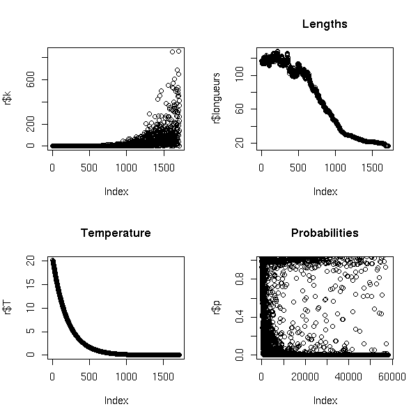
We can currently solve, exactly, TSP problems with several thousands of cities, by writing the problem as a "linear program". It is a bit tricky to describe, because there is an exponentially large number of constraints (namely, we want to exclude closed cycles, and we have one constraint for each possible cycle): we start to solve the problem without any constraint, we look at the constraints that are infringed (the cycles in the result), we explicitely add those constraints and we go on until we get a feasable solution.
TODO: give more details
After roaming the internet, I found "Concorde": it is a TSP solver (developed at Princeton, frrely useable for academic purposes) that relies on a linear programming solver such as QSopt (same licence) or CPlex (commercial and expensive).
http://www.tsp.gatech.edu/concorde.html
http://www.isye.gatech.edu/~wcook/qsopt/
http://www.ilog.com/products/cplex/

The documentation of the file formats:
http://www.informatik.uni-heidelberg.de/groups/comopt/software/TSPLIB95/DOC.PS
The website http://www.branchandcut.org/ lists Branch and Cut (this is one of the algorithms used to solve integer programs) software.
Symphony is an open source software to solve branc-and-cut problems such as the TSP. It also assumes we have a linear program solver such as CLP, Coin LP Solver (COIN, COmputational INfrasctructure for Operations Research, also open source, comes from IBM).
http://branchandcut.org/SYMPHONY/
http://www.coin-or.org/
Here is an example with "linkern", a program (part of concorde) that uses a heuristic to solve a TSP.
print.tsp <- function (x, d=dist(x), f="") {
  ## BEWARE: The documentation states "All explicit [weight] data is
  ##         integral"
  ## If the best tour has length 0, the problem may come from there.
  d <- round(as.dist(d))
  n <- dim(x)[1]
  cat("TYPE : TSP\n", file=f) # Creating the file
  cat("DIMENSION : ", file=f, append=T)
  cat(n, file=f, append=T)
  cat("\n", file=f, append=T)
  cat("EDGE_WEIGHT_TYPE : EXPLICIT\n", file=f, append=T)
  cat("EDGE_WEIGHT_FORMAT : UPPER_ROW\n", file=f, append=T)
  cat("DISPLAY_DATA_TYPE : NO_DISPLAY\n", file=f, append=T)
  cat("EDGE_WEIGHT_SECTION\n", file=f, append=T)
  cat(paste(as.vector(d), collapse=" "), file=f, append=T)
  cat("\n", file=f, append=T)
  cat("EOF\n", file=f, append=T)
}
tsp.plot.linkern <- function (x, d=dist(x), ...) {
  print.tsp(x, d, f="tmp.tsp")
  system(paste("./linkern", "-o", "tmp.tsp_result", "tmp.tsp"))
  ij <- 1+read.table("tmp.tsp_result", skip=1)[,1:2]
  xy <- prcomp(x)$x[,1:2]
  plot(xy, ...)
  segments( xy[,1][ ij[,1] ],
            xy[,2][ ij[,1] ],
            xy[,1][ ij[,2] ],
            xy[,2][ ij[,2] ],
            col='red' )
  ij
}

op <- par(mfrow=c(3,3), mar=.1+c(0,0,0,0))
for (i in 1:9) {
  n <- 50
  k <- 3
  x <- matrix(rnorm(n*k), nr=n, nc=k)
  tsp.plot.linkern(x, d=round(100*dist(x)), axes=F)
  box()
}
par(op)
Let us now try with Concorde.
tsp.plot.concorde <- function (x, d=dist(x), plot=T, ...) {
  print.tsp(x, d, f="tmp.tsp")
  system(paste("./concorde", "tmp.tsp"))
  i <- scan("tmp.sol")[-1]
  ij <- 1+matrix(c(i, i[-1], i[1]), nc=2)
  xy <- prcomp(x)$x[,1:2]
  if (plot) {
    plot(xy, ...)
    n <- dim(ij)[1]
    segments( xy[,1][ ij[,1] ],
              xy[,2][ ij[,1] ],
              xy[,1][ ij[,2] ],
              xy[,2][ ij[,2] ],
              col=rainbow(n) )
  }
  ij
}
op <- par(mfrow=c(3,3), mar=.1+c(0,0,0,0))
for (i in 1:9) {
  n <- 50
  k <- 3
  x <- matrix(rnorm(n*k), nr=n, nc=k)
  tsp.plot.concorde(x, d=round(100*dist(x)), axes=F)
  box()
}
par(op)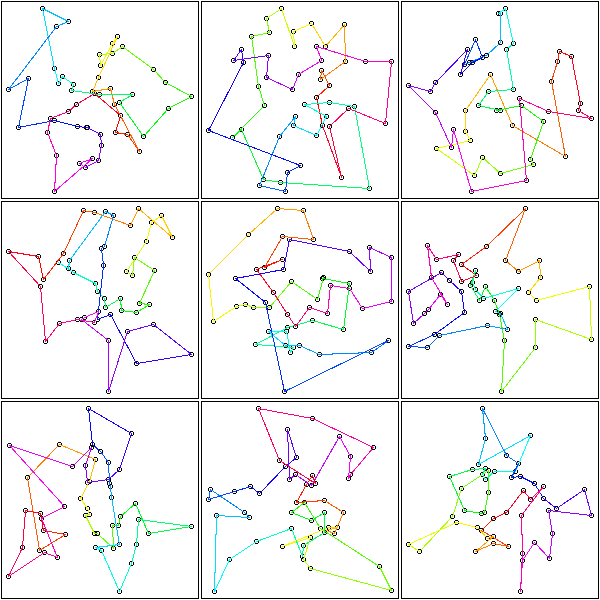
If we apply this to our simulated data, we get:
tsp.plot.concorde(t(data.broken.line))

There is one segment too many, because the algorith wants a closed path -- we want an open one.
With noisy data, it is even worse: the path goes on one direction and then comes back all the way.
tsp.plot.concorde(t(data.noisy.broken.line))
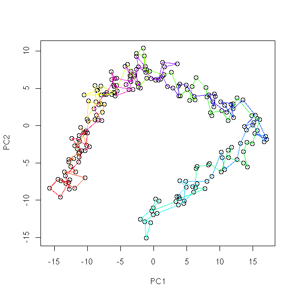
This is clearer if we smooth the curve:
x <- t(data.noisy.broken.line)
ij <- tsp.plot.concorde(x, plot=F)
xy <- prcomp(x)$x[,1:2]
y <- xy[ij[,1],]
x <- 1:dim(ij)[1]
plot(xy)
x1 <- predict(loess(y[,1]~x, span=.2))
x2 <- predict(loess(y[,2]~x, span=.2))
n <- length(x1)
segments(x1[-n], x2[-n], x1[-1], x2[-1], col=rainbow(n-1), lwd=3)

We can turn an open TSP program by adding a vertex whose distance to all the others is zero (or is the same).
print.open.tsp <- function (x, d=dist(x), f="") {
  ## BEWARE: The documentation states "All explicit [weight] data is
  ##         integral"
  ## If the best tour has length 0, the problem may come from there.
  d <- as.matrix(d)
  d <- cbind(0,rbind(0,d))
  d <- round(as.dist(d))
  n <- dim(x)[1] + 1
  cat("TYPE : TSP\n", file=f) # Creating the file
  cat("DIMENSION : ", file=f, append=T)
  cat(n, file=f, append=T)
  cat("\n", file=f, append=T)
  cat("EDGE_WEIGHT_TYPE : EXPLICIT\n", file=f, append=T)
  cat("EDGE_WEIGHT_FORMAT : UPPER_ROW\n", file=f, append=T)
  cat("DISPLAY_DATA_TYPE : NO_DISPLAY\n", file=f, append=T)
  cat("EDGE_WEIGHT_SECTION\n", file=f, append=T)
  cat(paste(as.vector(d), collapse=" "), file=f, append=T)
  cat("\n", file=f, append=T)
  cat("EOF\n", file=f, append=T)
}
tsp.plot.concorde.open <- function (x, d=dist(x), plot=T, smooth=F, span=.2,...) {
  print.open.tsp(x, d, f="tmp.tsp")
  system(paste("./concorde", "tmp.tsp"))
  i <- scan("tmp.sol")[-1]  # Remove the number of
  i <- i[-1]                # Remove the first node: 0
  ij <- matrix(c(i[-length(i)], i[-1] ), nc=2)
  xy <- prcomp(x)$x[,1:2]
  if (plot) {
    if (smooth) {
      y <- xy[ij[,1],]
      x <- 1:dim(ij)[1]
      plot(xy, ...)
      x1 <- predict(loess(y[,1]~x, span=span))
      x2 <- predict(loess(y[,2]~x, span=span))
      n <- length(x1)
      segments(x1[-n], x2[-n], x1[-1], x2[-1], col=rainbow(n-1), lwd=3)
    } else {
      plot(xy, ...)
      n <- dim(ij)[1]
      segments( xy[,1][ ij[,1] ],
                xy[,2][ ij[,1] ],
                xy[,1][ ij[,2] ],
                xy[,2][ ij[,2] ],
                col=rainbow(n) )
    }
  }
  ij
}
x <- t(data.noisy.broken.line)
tsp.plot.concorde.open(x)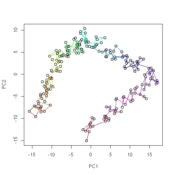
tsp.plot.concorde.open(x, smooth=T)

tsp.plot.concorde.open(t(data.curve), smooth=T)
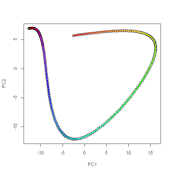
tsp.plot.concorde.open(t(data.noisy.curve), smooth=T)

tsp.plot.concorde.open(t(data.real), smooth=F)
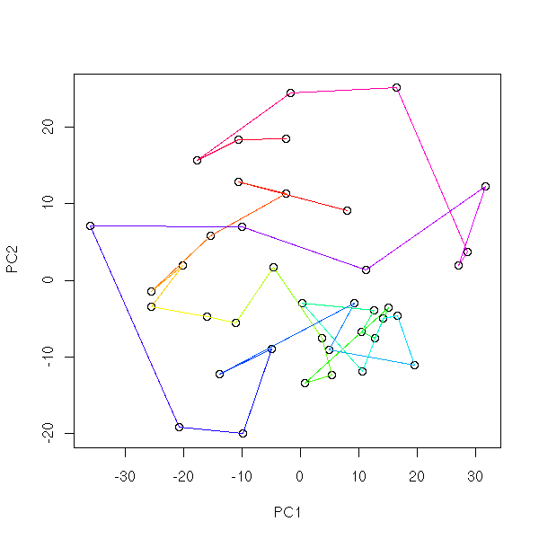
tsp.plot.concorde.open(t(data.real), smooth=T)

op <- par(mfrow=c(2,2))
for (s in c(.2, .3, .4, .5)) {
  tsp.plot.concorde.open(t(data.real), smooth=T, span=s)
}
par(op)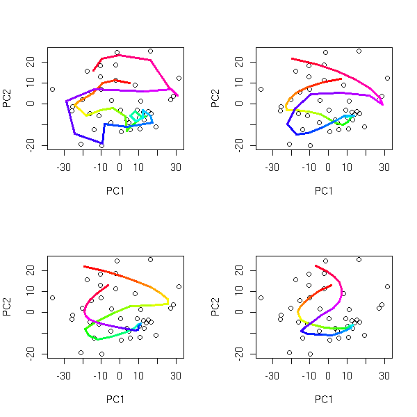
tsp.plot.concorde.open(data.real.3d, smooth=F)
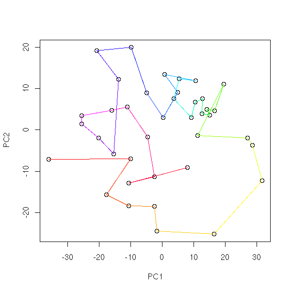
tsp.plot.concorde.open(data.real.3d, smooth=T)

tsp.plot.concorde.open(data.real.3d, smooth=T, span=.5)

Take our cloud of points, assign a mass to each so that they attract
each other. You can choose the law of attraction: for instance, a
force proportionnal to the inverse of the square of the distance, We
then simulate the evolution of this system (but not until
equilibrium: we stop before: after some time, the points seem to
form a curve).

This is one of the algorithms used to draw knots -- but is is rather
tricky to tune: if you make a mistake with the weights or the law of
attraction, you can get points that collapse on one another or that
go to infinity.

TODO: References?

There are several delicate choices:
1. The law of attraction
1bis. The dimension of the space (in which the points live and in
which we compute the distance) might have some importance.
2. The simulation of the evolution (not too fast, not too slow)
3. When do we stop?

Idea to decide when to stop:
Look at the ramification of the Minimal Spanning Tree (I define the
ramification of a tree as the number of nodes that are not on the
longest path -- it is easy to find: simply compute the matrix of
distances in the graph -- but there might be faster algorithms --
indeed:
  Remove the shortest edge among those leading to a leaf
  This creates a vertex of arity 2: fuse the two edges.
  Repeat until we are left with a single segment.
Yet another idea
Asign a random value to the index of each point of the cloud
This gives an order on the points
Consider the corresponding curve (broken line)
Smooth it.
Project the points on this curve and get a new value of the index.
Iterate
Yet another idea
Cluster the points into several classes
Find a segment for each of those classes
Try to glue those segments (how?)
Idea 1bis
TODO: svm if you know the index of each patient.
Add the computation time
Legends in my plots

For neural networks, present things a bit differently:
In-line algorithm, that always takes new data (this is easy, because
  we know how the data were obtained, get can ask for an infinite
  number of them)
Start with the linear PCA anc compare the neural-net implementation
  with the linear algebra one.

Optimization algorithms:
Start with a simple situation: a single segment, no noise, in
  dimension 2 (or even 1)
In particular this will help see if/where my code is wrong.

TODO: for the simulated data, divide the points into 4 groups, with
a colour for each. Thus, it will be clearer if we are supposed to
see something or not.
Ideally, we could also put all those plots in a single function that
we would call for all the examples.
TODO...
library(e1071)
?lca

library(poLCA)
?poLCA
The "ade4" package contains a lot of variants or applications of Principal Component Analysis.
library(help=ade4)
See also
library(help=pcurve)
Principal Component Analysis and the methods that stem from it are linear: if the data is not linear, the result may be meaningless.
http://nitro.biosci.arizona.edu/courses/EEB581-2004/handouts/Eigenstructure.pdf

This work is licensed under a Creative Commons Attribution-NonCommercial-ShareAlike 2.5 License.
Vincent Zoonekynd
<zoonek@math.jussieu.fr>
latest modification on Sat Jan 6 10:28:19 GMT 2007