Introduction to R

Features
Installing R
R: Documentation
Graphical interface -- R for non-statisticians and non-programmers
R: Some elementary functions

In this part, we give a bird's eye view of the software: what is its position with respect to other software for numeric computations? What are its advantages, its drawbacks? What can we do with it? What are its limitations? What is its syntax?

Features

Statistics vs Signal processing

It is a statistical software: contrary to other numerical computation software (Scilab, Octave),

http://www-rocq.inria.fr/scilab/
http://www.octave.org/

it already provides functions to perform non trivial statistical operations, be they classic (regression, logistic regression, analysis of variance (anova), decision trees, principal component analysis, etc.) or more modern (neural networks, bootstrap, generalized additive models (GAM), mixed models, etc.).

However, sometimes, in statistics, we use a lot of signal processing algorithms (Fourrier transform, wavelet transforms, etc.); if this is your case, you might find Scilab or Matlab more appropriate.

GUI -- or lack thereof

It is a real programming language, not a point-and-click software (in French I have a good neologism to describe those "point-and-click" programs: "cliquodromes" -- if someone knows of a good English translation, he is welcome): we are not limited by the software designers' imagination, we can use it to any means.

If you really need a simple and powerful GUI, have a look at R Commander, mentionned later in this document: it is a GUI that helps you learn the underlying language.

Speed issues

R is an interpreted language: the advantage, is that we spend less time writing code, the drawback is that the computations are slower -- but unless you wish to do real-time computations on the National Insurance files, taking into account the whole British population, or real-time computations involving billions of financial records, it is sufficiently fast.

If speed is really an issue, you can have a look at SAS (commercial, expensive, dating back to the mainframe era), DAP (free but far from complete: it was initially designed as a free replacement for SAS, but turned out to be a modest C library to perform statistical computations)

http://www.gnu.org/software/dap/dap.html

or you can program everything yourself (in C or C++), with the help of a few libraries

GSL (GNU Scientific Library), for special functions
(a good replacement for the ageing Numerical Recipes,
with a licence that actually allows you to use the software)
http://www.gnu.org/software/gsl/

LibSVM (Support Vector Machines)
http://www.csie.ntu.edu.tw/~cjlin/libsvm/

FFTW (Fast Fourier Transform)
http://www.fftw.org/
djbFFT (Fast Fourier Transform)
http://cr.yp.to/djbfft.html

IT++ (Signal processing)
http://itpp.sourceforge.net/

CLN (arbitrary precision)
http://www.ginac.de/CLN/
Core (Multi-precision library?)
http://www.cs.nyu.edu/exact/core_pages/

Gaul (Genetic algorithms)
http://gaul.sourceforge.net/
GALib (Genetic algorithms)
http://lancet.mit.edu/ga/

GTS (GNU Triangulated Surface library)
http://gts.sourceforge.net/

???
http://www.gnu.org/software/goose/goose.html

???
http://scythe.wustl.edu/scythe01/intro01-1.html

or (it is the approach I would advise) you can start to program in R, until you have a slow but correct program, profile your program (it means: find where it spends most of its time), try to change the algorithm so that it be faster and, if it fails, implement in C the most computation-intensive parts. If you try to optimize your program too early, you run the risk of either losing your time by optimizing parts of the implementation that have no real importance on the total time and getting a program with an awkward structure, very difficult to modify or extend -- or simply giving up your project before its completion.

Memory issues

There is another problem in R: it tends to load all the data into memory (this is slowly changing, starting with R version 2). For very large data, R might not be the best choice: I recently spoke to a statistician working with genetic data: their data were too large for R, too large for SAS and they had to resort to home-made programs. Yet, I said above, R might be a platform of choice for prototyping, i.e., to write the first versions of an application, while we know neither which algorithms to choose, nor how long the computations will take. Furthermore, as R can access most databases (some, such as PostgreSQL, even allow you to write stored procedures in R): you can store your data there and only retrieve the bits you need, when you need them. Personnaly, the first time I ran into memory problems once, I was playing with a time series containing several minutes of music.

If you have memory issues, you should also avoid Windows: it imposes further memory limitations -- indeed, if you read the R-help mailing list, all the people having memory issues are under Windows and their problems come from the operating system, not from R.

Graphics

R can produce graphics, but it is not a presentation software: for informative pictures, for graphical data exploration, it is fine, but if you want to use them in an advert, to impress or deceive your customers, you might have to process them through other software -- for instance, the title image of this document was created with R, PovRay and The Gimp.

http://www.gimp.org/
http://gimp-savvy.com/BOOK/index.html
http://gug.sunsite.dk/
http://www.povray.org/

Freedom

Finally, R is a free software ("free" as in "free speech" -- and also, incidentally, as in "free beer", but this is just a side effect). But beware: some (rare) libraries are not free but just "freely useable for non commercial purposes": be sure to read the licence.

Examples

Some people have started to set up R galleries:

http://addictedtor.free.fr/graphiques/
http://bg9.imslab.co.jp/Rhelp/
http://wiki.r-project.org/
http://fawn.unibw-hamburg.de/cgi-bin/Rwiki.pl?GraphGallery

Installing R

Windows

You should really consider Linux instead of Windows. People using R on Windows always have a lot of problems: especially memory problems (Windows specialists tell me that this operating system becomes unstable when a process wants to use more than 1Gb of memory -- and now that I use it at work, I can confirm the problems) and installation problems (if you want to install a package, you will have to find a binary version of it, for the very version of R you have installed -- alternatively, you can try to compile the packages from source, but this is very tricky, because Windows lacks all the tools for this: you end up installing Unix utilities on your Windows machine, but you will also run into version problems).

Not convinced?

> library(fortunes)
> fortune("install")

Benjamin Lloyd-Hughes: Has anyone had any joy getting the
rgdal package to compile under windows?  Roger Bivand: The
closest anyone has got so far is Hisaji Ono, who used MSYS
(http://www.mingw.org/) to build PROJ.4 and GDAL (GDAL
depends on PROJ.4, PROJ.4 needs a PATH to metadata files
for projection and transformation), and then hand-pasted
the paths to the GDAL headers and library into
src/Makevars, running Rcmd INSTALL rgdal at the Windows
command prompt as usual. All of this can be repeated, but
is not portable, and does not suit the very valuable
standard binary package build system for Windows. Roughly:
[points 1 to 5 etc omitted]

Barry Rowlingson: At some point the complexity of
installing things like this for Windows will cross the
complexity of installing Linux... (PS excepting live-Linux
installs like Knoppix)

   -- Benjamin Lloyd-Hughes, Roger Bivand and Barry Rowlingson
      R-help (August 2004)

Still not convinced? Well, good luck (you will need it). You can download a Windows version of R from

http://cran.r-project.org/bin/windows/base/

MacOS X

I am not familiar with MacOS, but you should not have any problem.

http://cran.r-project.org/

Linux

If you are new to Linux, you should first play around with a "live CD", i.e., a CD or DVD containing the whole operating system and useable without installing anything on your hard drive.

If you want one targeted to numerical computations and containing R, I suggest Quantian.

http://dirk.eddelbuettel.com/quantian.html

If you want a more general distribution, try Knoppix (I use it as a rescue disk, e.g., in case of password loss).

http://www.knopper.net/knoppix/index-en.html
http://www.oreilly.com/catalog/knoppixhks/

If you want a lot of eye-candy, have a look at eLive.

http://www.elivecd.org/

Once you are satisfied with one of those distributions, you can install Linux on your computer. Many people suggest Ubuntu (I have had a very bad experience with it, but you can assume I was unlucky); I was quite pleased when I last tried Suse; I used to use Mandriva but became dissatisfied with it. Many companies use Red Hat or its free, RedHat-sponsored equivalent, Fedora Core, mainly on their servers -- organizations using Linux on the desktop prefer Suse. To choose, check what people around you are using and take the same distribution: those people will be able to answer your questions.

http://distrowatch.com/table.php?distribution=ubuntu
http://distrowatch.com/table.php?distribution=suse
http://distrowatch.com/table.php?distribution=mandriva
http://distrowatch.com/table.php?distribution=redhat
http://distrowatch.com/table.php?distribution=fedora

I personnaly use Gentoo -- if you are not already an experienced Linux user, do not even think using it.

http://distrowatch.com/table.php?distribution=gentoo

Linux: Installing R on Mandriva

Just type

urpmi R-base R-bioconductor

That is all. No need to roam the web to find where you can download the software, no need to answer lengthy questions about where to install the software, no need to do anything yourself.

Linux: Installing R on Gentoo

Just type

emerge R

Linux: installing R from the sources

I proceed as follows:

# Installing R, from source

# A few required packages (when I currently use Gentoo Linux)
emerge lapack graphviz

wget http://cran.r-project.org/src/base/R-4/R-2.4.0.tar.gz
tar zxvf R-*.tar.gz
cd R-*/
./configure
make
make test
make install

# Installing the shared library libRmath (needed to
# compile some third-party programs, such as JAGS)
cd src/nmath/standalone
make
make install
echo /usr/local/lib >> /etc/ld.so.conf
ldconfig
cd ../../../../

# Installing ALL the CRAN packages
wget -r -l 1 -np -nc -x -k -E -U Mozilla -p -R zip www.stats.bris.ac.uk/R/src/contrib/
for i in www.stats.bris.ac.uk/R/src/contrib/*.tar.gz
do
  R CMD INSTALL $i
done

# Bioconductor
echo '
  source("http://www.bioconductor.org/getBioC.R")
  getBioC(groupName="all")
' | R --vanilla

echo /usr/lib/graphviz/ >> /etc/ld.so.conf
ldconfig
ln -s /usr/lib/graphviz/*.so* /usr/local/lib/ # Should not be necessary, but...

R: Documentation

First steps

The following document explains how to use R, progressively, at an elementary level (as long as the expressions "standard deviation" and "gaussian distribution" do not frighten you, it will be fine). Since I read it, this document became a book.

http://cran.r-project.org/doc/contrib/SimpleR.pdf
http://www.math.csi.cuny.edu/UsingR/

Here is the official introduction to R -- it is garanteed to be up to date.

http://cran.r-project.org/doc/manuals/R-intro.pdf

Another elementary document, with exercises, for German-speaking people.

http://cran.r-project.org/doc/contrib/s.pdf

RTFM

The reference manual is available under R: just type the name of the command whose reference you want prefixed by an interrogation mark.

?round

For reserved words or non-alphanumeric commands, use quotes.

?"for"
?"[["
?"[<-.data.frame"

If you do not know the command name (this happens very often), use "help.search" or "apropos".

help.search("stem")
apropos("stem")
RSiteSearch("stem")

The first one, "help.search", looks everywhere, especially in all the packages that are not loaded, while the second one, "help.search", looks in the search path, i.e., in all the functions and variables that are currently available. The last one looks on the R web site and on the R-help mailing list; a new tab will open in your browser.

https://stat.ethz.ch/pipermail/r-help/

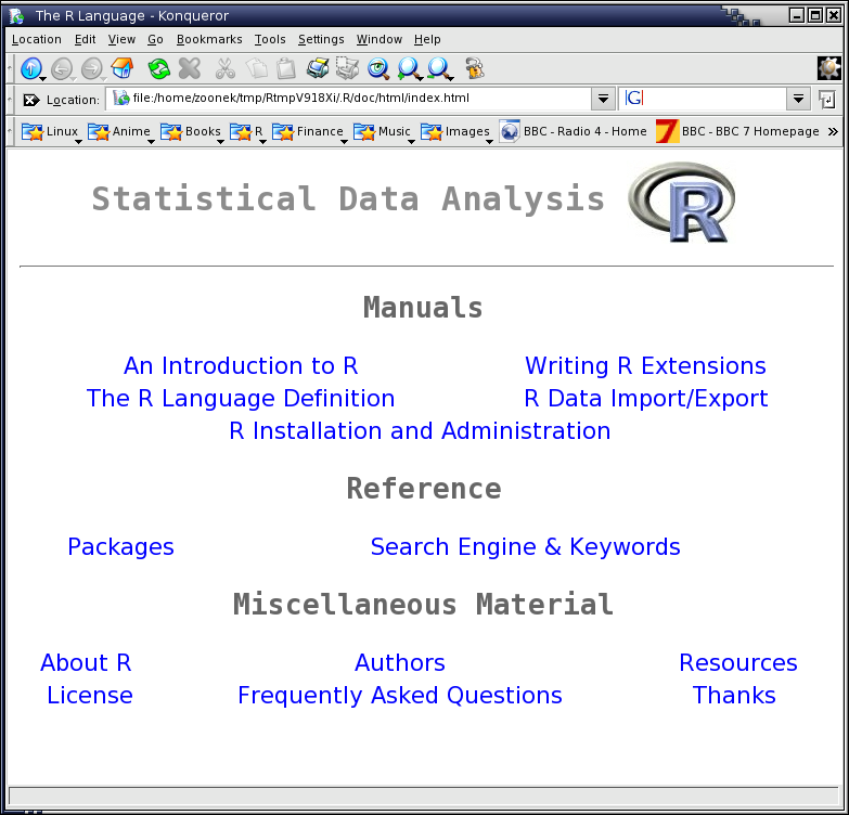
Some of you might prefer to read the manuals in HTML (R launches your default web browser -- in my case, konqueror).

help.start()

There are also a few PDF files in /usr/lib/R/library/*/doc/: it is sometimes a PDF version of the reference manual (when the file name is that of the library), but sometimes different, more pedagogic explainations, called "vignettes".

% cd /usr/local/lib/R/library/
% ls */doc/*pdf
AlgDesign/doc/AlgDesign.pdf
BHH2/doc/BHH2.pdf
Biobase/doc/Biobase.pdf
Biobase/doc/Bioconductor.pdf
Biobase/doc/HowTo.pdf
Biobase/doc/eSetMeta.pdf
Biobase/doc/esApply.pdf
Biobase/doc/eset.pdf
Biostrings/doc/Alignments.pdf
Biostrings/doc/Biostrings2Classes.pdf
Biostrings/doc/DNAStringVectorization.pdf
Biostrings/doc/matchPattern.pdf
BradleyTerry/doc/BradleyTerry-overview.pdf
BsMD/doc/BsMD.pdf
CDNmoney/doc/CDNmoney.pdf
CGIwithR/doc/CGIwithR-overview.pdf
CTFS/doc/CTFS.Chpt1.InstallingR.pdf
CTFS/doc/CTFS.Chpt2.AddressingObjects.pdf
CTFS/doc/CTFS.Chpt3.HelpPages.pdf
CTFS/doc/CTFS.Chpt4.FileStructure.pdf
CTFS/doc/CTFS.Chpt6.ReadWrite.pdf
CTFS/doc/CTFS.Chpt7.UsefulRFunctions.pdf
DBI/doc/DBI.pdf
DBI/doc/RS-DBI-origianl.pdf
DDHFm/doc/DDHFm.pdf
Devore6/doc/Devore6.pdf
GPArotation/doc/GPArotation.pdf
HSAUR/doc/Ch_analysing_longitudinal_dataI.pdf
HSAUR/doc/Ch_analysing_longitudinal_dataII.pdf
HSAUR/doc/Ch_analysis_of_variance.pdf
HSAUR/doc/Ch_cluster_analysis.pdf
HSAUR/doc/Ch_conditional_inference.pdf
HSAUR/doc/Ch_density_estimation.pdf
HSAUR/doc/Ch_errata.pdf
HSAUR/doc/Ch_introduction_to_R.pdf
HSAUR/doc/Ch_logistic_regression_glm.pdf
HSAUR/doc/Ch_meta_analysis.pdf
HSAUR/doc/Ch_multidimensional_scaling.pdf
HSAUR/doc/Ch_multiple_linear_regression.pdf
HSAUR/doc/Ch_principal_components_analysis.pdf
HSAUR/doc/Ch_recursive_partitioning.pdf
HSAUR/doc/Ch_simple_inference.pdf
HSAUR/doc/Ch_survival_analysis.pdf
HSAUR/doc/preface.pdf
LMGene/doc/LMGene.pdf
MasterBayes/doc/MasterBayes.Tutorial.pdf
Matrix/doc/Comparisons.pdf
Matrix/doc/Introduction.pdf
POT/doc/guide.pdf
ProbForecastGOP/doc/vignette.pdf
QCAGUI/doc/Getting-Started-with-the-Rcmdr.pdf
R.oo/doc/Bengtsson.pdf
R.rsp/doc/R.rsp-package.pdf
R2HTML/doc/R2HTML.pdf
R2WinBUGS/doc/R2WinBUGS.pdf
R2WinBUGS/doc/benzolsw.pdf
R2WinBUGS/doc/countssw.pdf
R2WinBUGS/doc/expectedsw.pdf
R2WinBUGS/doc/plot.pdf
RBGL/doc/RBGL.pdf
RBGL/doc/filedep.pdf
RGtk2/doc/design.pdf
RGtk2/doc/overview2.pdf
RII/doc/RIIoverview.pdf
RLMM/doc/RLMM.pdf
ROC/doc/ROCnotes.pdf
RUnit/doc/RUnit.pdf
Rcmdr/doc/Getting-Started-with-the-Rcmdr.pdf
RcppTemplate/doc/RcppAPI.pdf
Rgraphviz/doc/Rgraphviz.pdf
Rgraphviz/doc/layingOutPathways.pdf
Rigroup/doc/Rigroup.pdf
Ruuid/doc/Ruuid.pdf
SAGx/doc/samroc-ex.pdf
SASmixed/doc/Usinglme.pdf
SharedHT2/doc/SharedHT2.pdf
SparseM/doc/SparseM.pdf
StatDataML/doc/StatDataML.pdf
TwoWaySurvival/doc/paper.pdf
UNF/doc/UNF_vignette.pdf
accuracy/doc/accuracy_vignette.pdf
adehabitat/doc/classes.pdf
affy/doc/affy.pdf
affy/doc/builtinMethods.pdf
affy/doc/customMethods.pdf
affy/doc/dealing_with_cdfenvs.pdf
affy/doc/vim.pdf
affyPLM/doc/AffyExtensions.pdf
affyPLM/doc/QualityAssess.pdf
affyPLM/doc/ThreeStep.pdf
affydata/doc/affydata.pdf
amap/doc/amap.pdf
annaffy/doc/annaffy.pdf
annotate/doc/annotate.pdf
annotate/doc/chromLoc.pdf
annotate/doc/prettyOutput.pdf
annotate/doc/query.pdf
annotate/doc/useDataPkgs.pdf
annotate/doc/useHomology.pdf
annotate/doc/useProbeInfo.pdf
approximator/doc/apprex.pdf
arules/doc/arules.pdf
aster/doc/design.pdf
aster/doc/ktp.pdf
aster/doc/trunc.pdf
aster/doc/tutor.pdf
asypow/doc/asypow.pdf
asypow/doc/asypow.statlib.pdf
backtest/doc/backtest.pdf
bayesSurv/doc/INDEX.pdf
bayesSurv/doc/Komarek_Lesaffre_2005.pdf
bayesSurv/doc/Komarek_Lesaffre_2006.pdf
bayesSurv/doc/cgd.pdf
bayesSurv/doc/tandmobCS.pdf
bayesSurv/doc/tandmobMixture.pdf
bayesSurv/doc/tandmobPA.pdf
bayesm/doc/Some_Useful_R_Pointers.pdf
bayesm/doc/Tips_On_Using_bayesm.pdf
bayesm/doc/bayesm-manual.pdf
bim/doc/bim.pdf
bindata/doc/artdatagen.pdf
binom/doc/sundar_dorai-raj_jsm_2006.pdf
calibrate/doc/CalibrationGuide.pdf
calibrator/doc/calex.pdf
chemCal/doc/chemCal.pdf
clue/doc/clue.pdf
clustvarsel/doc/varsel.vignette.pdf
clustvarsel/doc/vignplot1.pdf
coin/doc/LegoCondInf.pdf
coin/doc/coin.pdf
compositions/doc/UsingCompositions.pdf
cond/doc/Rnews-paper.pdf
copula/doc/copula.pdf
ctv/doc/ctv-howto.pdf
depmix/doc/depmix-intro.pdf
diveMove/doc/diveMove.pdf
dlm/doc/dlm.pdf
dr/doc/drdoc.pdf
drc/doc/drc.pdf
dse1/doc/dse-guide.pdf
dse1/doc/dse1.pdf
dse2/doc/dse2.pdf
e1071/doc/svm.pdf
e1071/doc/svmdoc.pdf
edd/doc/HOWTO-edd-compare.pdf
edd/doc/HOWTO-edd.pdf
edd/doc/eddDetails.pdf
emulator/doc/emulex.pdf
evd/doc/guide22.pdf
evdbayes/doc/guide.pdf
exactLoglinTest/doc/exactLoglinTest.pdf
fda/doc/FDAfuns.pdf
feature/doc/feature.pdf
femmeR/doc/femmeR.pdf
filehash/doc/filehash.pdf
flexmix/doc/flexmix-intro.pdf
fuzzyRankTests/doc/design.pdf
gWidgets/doc/addingToolkit.pdf
gWidgets/doc/gWidgets.pdf
gamlss/doc/gamlss-R-help-files.pdf
gamlss/doc/gamlss-manual.pdf
gap/doc/gap.pdf
gbm/doc/gbm.pdf
gbm/doc/oobperf2.pdf
gbm/doc/shrinkage-v-iterations.pdf
gcrma/doc/gcrma2.0.pdf
gdata/doc/gregmisc.pdf
genefilter/doc/howtogenefilter.pdf
genefilter/doc/howtogenefinder.pdf
geneplotter/doc/byChroms.pdf
geneplotter/doc/visualize.pdf
genetics/doc/LD.pdf
genetics/doc/genetics_article.pdf
geoRglm/doc/geoRglmintro.pdf
ggplot/doc/introduction.pdf
ggplot/doc/writing-grob-functions.pdf
globaltest/doc/GlobalTest.pdf
gnm/doc/gnmOverview.pdf
gplots/doc/BalloonPlot.pdf
gpls/doc/gpls.pdf
graph/doc/clusterGraph.pdf
graph/doc/graph.pdf
graph/doc/graphAttributes.pdf
grid/doc/displaylist.pdf
grid/doc/frame.pdf
grid/doc/grid.pdf
grid/doc/grobs.pdf
grid/doc/interactive.pdf
grid/doc/locndimn.pdf
grid/doc/moveline.pdf
grid/doc/nonfinite.pdf
grid/doc/plotexample.pdf
grid/doc/rotated.pdf
grid/doc/saveload.pdf
grid/doc/sharing.pdf
grid/doc/viewports.pdf
gridBase/doc/gridBase-complex.pdf
gridBase/doc/gridBase-multiplot.pdf
gridBase/doc/gridBase.pdf
gstat/doc/gstat.pdf
hapassoc/doc/hapassoc.pdf
haplo.stats/doc/help.haplo.stats.pdf
haplo.stats/doc/manualHaploStats.pdf
hexbin/doc/hexagon_binning.pdf
hierfstat/doc/hierfstat.pdf
hopach/doc/MSS.pdf
hopach/doc/hopachManuscript.pdf
hwde/doc/hwde.pdf
intcox/doc/aneur_km.pdf
intcox/doc/aneur_para.pdf
intcox/doc/comb1einzel.pdf
intcox/doc/intcox.pdf
ipred/doc/ipred-examples.pdf
kernlab/doc/kernlab.pdf
kinship/doc/releasep.pdf
ks/doc/kde.pdf
laser/doc/laser_input.pdf
lasso2/doc/Manual-wo-help.pdf
ldDesign/doc/assoc_bfdesign.pdf
ldbounds/doc/ldbounds.pdf
limma/doc/limma.pdf
limma/doc/usersguide.pdf
lme4/doc/Implementation.pdf
lmtest/doc/lmtest-intro.pdf
locfdr/doc/locfdr-example-Compute-local-fdr.pdf
locfdr/doc/locfdr-example.pdf
logcondens/doc/logcondens_vignette.pdf
maanova/doc/hckidney.pdf
maanova/doc/maanova.pdf
maanova/doc/vgprofile.pdf
makecdfenv/doc/makecdfenv.pdf
marg/doc/Rnews-paper.pdf
marray/doc/ExampleHTML.pdf
marray/doc/marray.pdf
marray/doc/marrayClasses.pdf
marray/doc/marrayClassesShort.pdf
marray/doc/marrayInput.pdf
marray/doc/marrayNorm.pdf
marray/doc/marrayPlots.pdf
marray/doc/widget1.pdf
matchprobes/doc/matchprobes.pdf
maxstat/doc/maxstat.pdf
mboost/doc/SurvivalEnsembles.pdf
mboost/doc/mboost_illustrations.pdf
mcmc/doc/demo.pdf
mcmc/doc/metrop.pdf
mfp/doc/mfp.pdf
mice/doc/Manual.pdf
mitools/doc/smi.pdf
mlmRev/doc/MlmSoftRev.pdf
mlmRev/doc/StarData.pdf
monoProc/doc/monoproc.pdf
msm/doc/msm-manual.pdf
multcomp/doc/Rmc.pdf
multtest/doc/MTP.pdf
multtest/doc/MTPALL.pdf
multtest/doc/multtest.pdf
mvtnorm/doc/MVT_Rnews.pdf
nlreg/doc/Rnews-paper.pdf
npmlreg/doc/npmlreg-manual.pdf
npmlreg/doc/npmlreg-v.pdf
numDeriv/doc/numDeriv.pdf
odfWeave/doc/RnewsExample.pdf
odfWeave/doc/RnewsOut.pdf
odfWeave/doc/odfWeave.pdf
optmatch/doc/listOfDistancesHowTo.pdf
optmatch/doc/mahalanobisMatching.pdf
optmatch/doc/optmatch.pdf
orientlib/doc/orientlib_paper.pdf
panel/doc/Panel-users-guide.pdf
partsm/doc/partsm.pdf
party/doc/MOB.pdf
party/doc/party.pdf
pastecs/doc/pastecs.pdf
pcalg/doc/Sweave-pcalg.pdf
plm/doc/baltagi.pdf
pmg/doc/pmg.pdf
poLCA/doc/poLCA-manual.pdf
polyapost/doc/pp1.pdf
portfolio/doc/matching_portfolio.pdf
portfolio/doc/portfolio.pdf
portfolio/doc/tradelist.pdf
powell/doc/NA2000_14.pdf
powell/doc/NA2002_02.pdf
pps/doc/pps-ug.pdf
proto/doc/cloning3.pdf
proto/doc/proto.pdf
proto/doc/protoref.pdf
proto/doc/test.pdf
qtlbim/doc/hyperpaper.pdf
qtlbim/doc/hyperslide.pdf
qtlbim/doc/qtlbim.pdf
qtlbim/doc/scan.pdf
quantreg/doc/rq.pdf
qvalue/doc/manual.pdf
qvalue/doc/pHist.pdf
qvalue/doc/qHist.pdf
qvalue/doc/qPlots.pdf
qvalue/doc/qvalue.pdf
rake/doc/rake-manual.pdf
random/doc/random-essay.pdf
random/doc/random-intro.pdf
relaimpo/doc/ChangeLog.pdf
relaimpo/doc/relaimpo_vignette.pdf
reposTools/doc/reposClient.pdf
reposTools/doc/reposServer.pdf
reshape/doc/introduction.pdf
resper/doc/huber-sim.pdf
reweight/doc/reweight-presentation.pdf
rhosp/doc/rhosp.pdf
rmetasim/doc/Using_Rmetasim.pdf
rmetasim/doc/islandtheta.pdf
rmetasim/doc/mismatch.pdf
rmetasim/doc/struct.pdf
rv/doc/rv.pdf
sandwich/doc/sandwich.pdf
scape/doc/dsc.pdf
scatterplot3d/doc/barplot.pdf
scatterplot3d/doc/binorm.pdf
scatterplot3d/doc/business.pdf
scatterplot3d/doc/colorcube.pdf
scatterplot3d/doc/drill1.pdf
scatterplot3d/doc/drill2.pdf
scatterplot3d/doc/elements.pdf
scatterplot3d/doc/helix.pdf
scatterplot3d/doc/hemisphere.pdf
scatterplot3d/doc/meta.pdf
scatterplot3d/doc/residuals.pdf
scatterplot3d/doc/s3d.pdf
seqinr/doc/seqinr_1_0-6.pdf
setRNG/doc/setRNG.pdf
siggenes/doc/siggenes.pdf
smoothSurv/doc/smmr-paper.pdf
sp/doc/sp.pdf
spatstat/doc/Intro.pdf
spatstat/doc/Quickref.pdf
spdep/doc/auckland.pdf
spdep/doc/sids.pdf
strucchange/doc/strucchange-intro.pdf
survBayes/doc/survBayes.pdf
surveillance/doc/flowchart.pdf
surveillance/doc/vignette.pdf
survey/doc/domain.pdf
survey/doc/epi.pdf
survey/doc/phase1.pdf
survey/doc/survey.pdf
systemfit/doc/vignette_systemfit.pdf
tframe/doc/tframe.pdf
tgp/doc/as.pdf
tgp/doc/exp.pdf
tgp/doc/fried.pdf
tgp/doc/linear.pdf
tgp/doc/moto.pdf
tgp/doc/sin.pdf
tgp/doc/tgp.pdf
tkWidgets/doc/importWizard.pdf
tkWidgets/doc/tkWidgets.pdf
trust/doc/trust.pdf
tsDyn/doc/tsDyn.pdf
tsfa/doc/tsfa.pdf
twang/doc/twang.pdf
ump/doc/design.pdf
vars/doc/vars.pdf
vcd/doc/labeling.pdf
vcd/doc/shading.pdf
vcd/doc/spacing.pdf
vcd/doc/struc.pdf
vcd/doc/strucplot.pdf
vegan/doc/partitioning.pdf
vegan/doc/vegan-FAQ.pdf
vsn/doc/convergence.pdf
vsn/doc/vsn.pdf
widgetTools/doc/widget.pdf
widgetTools/doc/widgetTools.pdf
wnominate/doc/wnominate.pdf
zipfR/doc/zipfr-tutorial.pdf
zoo/doc/zoo-quickref.pdf
zoo/doc/zoo-refcard.pdf
zoo/doc/zoo.pdf

CRAN Task Views

Most users will start to use R with a given application in mind, or at least, with a given domain in mind. This can be troublesome, because a given statistical procedure can be known under completely different names in different domains. Furthermore, some statistical procedures (or plots) will be used extremely often in a domain, to the point of being considered elementary, while it will be so rare in others that hardly anyone knows it.

To avoid those problems and directly jump to the packages and functions you need for your study, have a look at the CRAN Task Views: these are commented lists of R packages tailored for some domains.

http://cran.r-project.org/src/contrib/Views/

Graphics

The following document (very enlightening, even if it is written in a language I cannot read -- probably spanish) explains in details what kinds of graphics R can produce. At least, browse through it.

http://cran.r-project.org/doc/contrib/grafi3.pdf

The pictures in the manual

I said earlier that an HTML version of the manual was available (look in /usr/lib/R/), but it lacks the illustrations... (The development team is aware of the problem and it may be tackled in the near future.) The following web site has added them:

http://bg9.imslab.co.jp/Rhelp/

You can create them yourself, as follows.

#! perl -w
use strict;
my $n = 0;
  
# Writing R files
mkdir "Rdoc" || die "Cannot mkdir Rdoc/: $!";
my @libraries= `ls lib/R/library/`;
foreach my $lib (@libraries) {
  chomp($lib);
  print STDERR "Processing library \"$lib\"\n";
  print STDERR `pwd`;
  my @pages = grep /\.R$/, `ls lib/R/library/$lib/R-ex/`;
  chdir "Rdoc" || die "Cannot chdir to Rdoc: $!";
  mkdir "$lib" || die "Cannot mkdir $lib: $!";
  chdir "$lib" || die "Cannot chdir to $lib: $!";
  open(M, '>', "Makefile") || die "Cannot open Makefile for writing: $!";
  print M "all:\n";
  foreach my $page (@pages) {
    chomp($page);
    print STDERR "  Processing man page \"$page\" in library \"$lib\"\n";
    my $res = "";
    $res .= "library($lib)\n";
    $res .= "library(lattice)##VZ##\n";
    $res .= "library(nlme)##VZ##\n";
    $res .= "library(MASS)##VZ##\n";
    $res .= "identify <- function (...) {}##VZ##\n";
    $res .= "x11()##VZ##\n";
    open(P, '<', "../../lib/R/library/$lib/R-ex/$page") || 
      die "Cannot open lib/R/library/$lib/R-ex/$page for reading: $!";
    # Tag the lines where we must copy the screen (between two commands)
    while(<P>) {
      s/^([^ #}])/try(invisible(dev.print(png,width=600,height=600,bg="white",filename="doc$n.png")))##VZ##\n$1/
        && $n++;
      $res .= $_;
    }
    $res .= "try(invisible(dev.print(png,width=600,height=600,bg=\"white\",filename=\"doc$n.png\")))##VZ##\n"; $n++;
    close P;
    # We discard the line in the following cases:
    #   The previous line ends with a comma, an opening bracket, an "equal" sign
    $res =~ s/[,(=+]\s*\n.*##VZ##.*?\n/,\n/g;
    # The previous line is empty
    $res =~ s/^\s*\n.*##VZ##.*\n/\n/gm;
    # The previous line only contains a comment
    $res =~ s/^(\s*#.*)\n.*##VZ##.*\n/$1\n/gm;
    # The nest line starts with a {    TODO: check (boot / abc.ci)
    $res =~ s/^.*##VZ##.*\n\s*\{/\{/gm;
    # We write the corresponding number
    $res =~ s/doc([0-9]).png/doc00000$1.png/g;
    $res =~ s/doc([0-9][0-9]).png/doc0000$1.png/g;
    $res =~ s/doc([0-9][0-9][0-9]).png/doc000$1.png/g;
    $res =~ s/doc([0-9][0-9][0-9][0-9]).png/doc00$1.png/g;
    $res =~ s/doc([0-9][0-9][0-9][0-9][0-9]).png/doc0$1.png/g;
    open(W, ">", "${lib}_${page}") || die "Cannot open ${lib}_${page} for writing: $!";
    print W $res;
    close W;
    print M "\tR --vanilla <${lib}_${page} >${lib}_${page}.out\n";
    my $p = $page; 
    $p =~ s/\.R$//;
    system 'cp', "../../lib/R/library/$lib/html/$p.html", "${lib}_$p.html";
  }
  print M "\ttouch all\n";
  close(M);
  chdir "../../" || die "Cannot chdir to ../../: $!";
}

we compile them (it should take a few hours: for some packages, it may crash).

cd Rdoc/
for i in *
do
  (
    cd $i
    make
  )
done

I prefer to parallelize all this:

\ls -d */ | perl -p -e 's/(.*)/cd $1; make/' | perl fork.pl 5

where fork.pl allows you to launch several processes at the same time, but not too many:

#! /usr/bin/perl -w
use strict;
my $MAX_PROCESSES = shift || 10;
use Parallel::ForkManager;
my $pm = new Parallel::ForkManager($MAX_PROCESSES);
while(<>){
  my $pid = $pm->start and next; 
  system($_);
  $pm->finish; # Terminates the child process
}

We clean the PNG files thus generated and we write the HTML files,

for i in */
do
  (
    cd $i
    perl ../do.it_2.pl
  )
done

Where do.it_2.pl contains:

#! perl -w
use strict;
  
# Delete the empty or duplicated PNG files
print STDERR "Computing checksums\n";
use Digest::MD5 qw(md5);
my %checksum;
foreach my $f (sort(<*.png>)) {
  if( -z $f ) {
    unlink $f;
    next;
  }
  local $/;
  open(F, '<', $f) || warn "Cannot open $f for reading: $!";
  my $m = md5(<F>);
  close F;
  if( exists $checksum{$m} ){
    unlink $f;
  } else {
    $checksum{$m} = $f;
  }
}
  
# Turn all this into HTML
print STDERR "Converting to HTML\n";
open(HTML, '>', "ALL.html") || warn "Cannot open ALL.html for writing: *!";
select(HTML);
print "<html>\n";
print "<head><title>R</title></head>\n";
print "<body>\n";
foreach my $f (<*.R.out>) {
  my $page = $f;
  $page =~ s/\.R.out$//;
  # Read the initial HTML file
  if( open(H, '<', "$page.html") ){
    my $a = join '', <H>;
    close H;
    $a =~ s#^.*?<body>##gsi;
    $a =~ s#<hr>.*?$##gsi;
    print $a;
  } else {
    warn "Cannot open $page.html for reading: $!";
  }
  open(F, '<', $f) || warn "Cannot open $f for reading: $!";
  #print "<h1>$f</h1>\n";
  print "<h2>Worked out examples</h2>\n";
  print "<pre>\n";
  my $header=1;
  while(<F>) {
    if($header) {
      $header=0 if m/to quit R/;
      next;
    }
    if( m/(doc.*png).*##VZ##/ ){
      my $png = $1;
      next unless -f $png;
      print "</pre>\n";
      print "<img width=600 height=600 src=\"$png\">\n";
      print "<pre>\n";
    }
    next if m/##VZ##/;
    next if m/^>\s*###---/;
    next if m/^>\s*##\s*___/;
    next if m/^>\s*##\s*(alias|keywords)/i;
    s/\&/\&amp;/g;
    s/</&lt;/g;
    print;
  }
  close F;
  print "</pre>\n";
  print "<hr>\n";
}
print "</body>\n";
print "</html>\n";
close HTML;

For an unknown reason, the PNG files have a transparent background: I turn it into a white background with ImageMagick (the white.png file is a white PNG file, of the same size, 600x600, created with The Gimp) -- here as well, it is pretty long...

for i in */*png
do
  echo $i
  composite $i white.png $i
done

I do not take into account the potential links in the HTML files (not very clean, but...).

perl -p -i.bak -e 's#<a\s.*?>##gi; s#</a>##gi' **/ALL.html

The HTML files should rather be called index.html:

rename 's/ALL.html/index.html/' */ALL.html

where "rename" is the program:

#!/usr/bin/perl -w
use strict;
my $reg = shift @ARGV;
foreach (@ARGV) {
  my $old = $_;
  eval "$reg;";
  die $@ if $@;
  rename $old, $_;
}

here is a very small piece of the result (2.7Mb, 268 pictures, while the whole documentation reaches 93Mb and 2078 images -- this was R 1.6 -- it is probably much more now).

Rdoc/index.html

In particular, one might be interested in the packages whose documentation contains the highest number of graphics.

% find -name "*.png"  | perl -p -e 's#^\./##;s#/.*##' | sort | uniq -c | sort -n | tail -20
   26 sm
   27 cluster
   29 ade4
   29 nls
   29 spatial
   31 mgcv
   34 car
   38 cobs
   41 MPV
   44 mclust
   45 MASS
   45 vcd
   49 grid
   60 gregmisc
   64 pastecs
   70 qtl
   77 splancs
   88 strucchange
   90 waveslim
  113 spdep

Graphical interface -- R for non-statisticians and non-programmers

ESS

It is the statistical mode of Emacs (it may be automatically installed with (X)Emacs: under Mandriva Linux (formerly Mandrake), it is with XEmacs, it is not with Emacs). One may then edit code with automatic indentication and syntax highlighting (Emacs recognises the files from their extension).

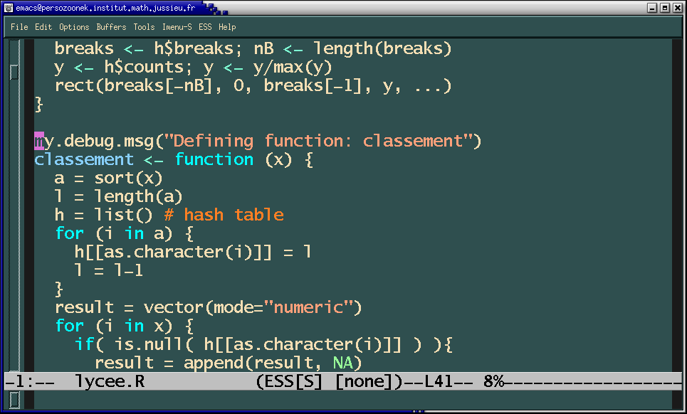
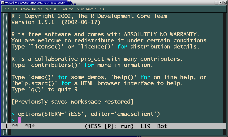
You can even run R under Emacs (M-x R).

Windows-specific stuff

Under windows, R has a graphical interface -- it is just a makeshift replacement to accomodate for the lack of a decent terminal under Windows: it is not a menu-driven interface.

You might still need a text editor, though. Some people advise Tinn-R, an R-aware simple text editor.

http://www.sciviews.org/Tinn-R/

R Commander

This really is a menu-oriented interface to R, that allows you to navigate through your data sets, to perform simple statistical analyses,

If you do not need anything beyond regression (but if you need all the graphical diagnostics that should be performed after a regression) and simple tests, or simply, if you have to teach statistics to non-statisticians and non-programmers, it seems to me an excellent choice. Users who later want to unleash the full power of R as a real programming language will face a gentle transition: R Commander displays all the commands that are run in the background to perform the tests and regressions and to produce the plots.

If you want to provide a GUI tailored to a certain domain, providing analyses specific to it, it is a good starting point: you can add you own menus to the interface.

Several projects have started to do this, in specific areas, for instance fBrowser, for finance and econophysics, in Rmetrics, and GEAR, for introductory econometrics.

Zelig

One big problem with R, and one big difference with menu-driven software, is that you never know where the feature you need is -- and this is even more true if you do not know the feature in question (you cannot wander through the menus). The typical example is "logistic regression": the main function to perform logistic regression is "glm". This stands for "Generalized Linear Models" (do not worry, you are not supposed to know what it is) and the manual page does not even give an example of a logistic regression. If you know the theory behind logistic regression, if you know that it is a special case of GLM, you might be fine -- but most users do not know, or do not want to, and should not need to.

The Zelilg library fulfils the needs of such people by providing a simplified and uniform interface to most statistical procedures.

http://gking.harvard.edu/zelig/

Basically, you only need to know five functions: "zelig" (to fit a model), "setx" to change the data (for predictions), "sim" to simulate new values (i.e., to predict the values), "summary" and "plot".

TODO: Give an example...

library(Zelig)
d <- data.frame(
  y = crabs$sp,
  x1 = crabs$FL,
  x2 = crabs$RW
)
r <- zelig( y ~ x1 + x2, model="probit", data=d )
summary(r)
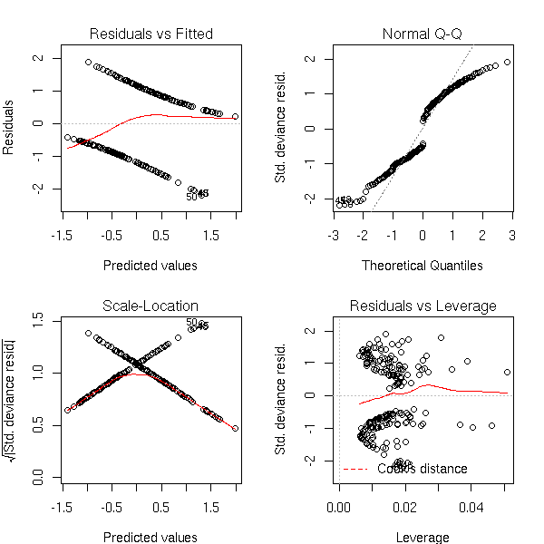
op <- par(mfrow=c(2,2), mar=c(4,4,3,2))
plot(r)
par(op)

NOT RUN %G
N <- dim(d)[1]
new.x1 <- rnorm( N, mean(d$x1), sd(d$x1) )
new.x2 <- rnorm( N, mean(d$x2), sd(d$x2) )
## BUG in Zelig?
s <- sim(r, setx(r, data=data.frame(x1=new.x1, x2=new.x2)))
plot(s)
%--

You can choose the model among the following list:

To predict a quantitative variable:
  ls      Least Squares
  normal  (almost the same)
  gamma   Gamma regression

To predict a binary variable:  
  logit   Logistic regression
  relogit Logistic regressioni for rare events
  probit  Probit regression

To predict two binary variables: 
  blogit  Bivariate logistic regression
  bprobit Bivariate probit regression

To predict a qualitative variable
  mlogit  Multinomial logistic

To predict an ordered qualitative variable: 
  ologit  Ordinal logistic regression
  oprobit Ordinal probit regression

To predict count data:
  poisson Poisson regression
  negbin  Negative binomial regression (as Poisson regression, but
          with more dispersed observations)

To predict survival data:
  exp      Exponential model (the hazard rate is constant)
  weibull  Weibull model (the hazard rate increases with time)
  lognorm  Log-normal model (the hazard rate increases and then decreases)

The unification of the various statistical models is a great thing, but this library does not put enough emphasis on the graphics to be looked at before, during and after the analysis -- as opposed to R Commander.

SciViews

An other user-friendly interface to R.

http://www.sciviews.org/SciViews-R/

JGR (pronounce "jaguar")

Yet another GUI, in Java.

http://stats.math.uni-augsburg.de/JGR/

R: Some elementary functions

In this part, we present the simplest functions of R, to allow you to read data (or to simulate them -- it is so easy, you end up doing it all the time, to check if your algorithms are correct (i.e., if they behave as expected if the assumptions you made on your data are satisfied) before applying them to real data) and to numerically or graphically explore them.

In the following, the ">" at the begining of the lines is R's prompt -- you should not type it --, the [1] at the begining of some lines is part or R's answers.

Statistics, computations:

>            # 20 numbers, between 0 and 20
>            # rounded at 1e-1
> x <- round(runif(20,0,20), digits=1)  
> x
 [1] 10.0  1.6  2.5 15.2  3.1 12.6 19.4  6.1  9.2 10.9  9.5 14.1 14.3 14.3 12.8
[16] 15.9  0.1 13.1  8.5  8.7

> min(x)
[1] 0.1

> max(x)
[1] 19.4

> median(x)  # median
[1] 10.45

> mean(x)    # mean
[1] 10.095

> var(x)     # variance
[1] 27.43734

> sd(x)      # standard deviation 
[1] 5.238067

> sqrt(var(x))
[1] 5.238067

> rank(x)    # rank
 [1] 10.0  2.0  3.0 18.0  4.0 12.0 20.0  5.0  8.0 11.0  9.0 15.0 16.5 16.5 13.0
[16] 19.0  1.0 14.0  6.0  7.0

> sum(x)
[1] 201.9

> length(x)
[1] 20

> round(x)
 [1] 10  2  2 15  3 13 19  6  9 11 10 14 14 14 13 16  0 13  8  9

> fivenum(x)     # quantiles
[1]  0.10  7.30 10.45 14.20 19.40

> quantile(x)    # quantiles (different convention)
   0%   25%   50%   75%  100%
 0.10  7.90 10.45 14.15 19.40

> quantile(x, c(0,.33,.66,1))
    0%    33%    66%   100%
 0.100  8.835 12.962 19.400

> mad(x)         # normalized mean deviation to the median ("median average distance"
[1] 5.55975

> cummax(x)
 [1] 10.0 10.0 10.0 15.2 15.2 15.2 19.4 19.4 19.4 19.4 19.4 19.4 19.4 19.4 19.4
[16] 19.4 19.4 19.4 19.4 19.4

> cummin(x)
 [1] 10.0  1.6  1.6  1.6  1.6  1.6  1.6  1.6  1.6  1.6  1.6  1.6  1.6  1.6  1.6
[16]  1.6  0.1  0.1  0.1  0.1

> cor(x,sin(x/20))    # correlation
[1] 0.997286

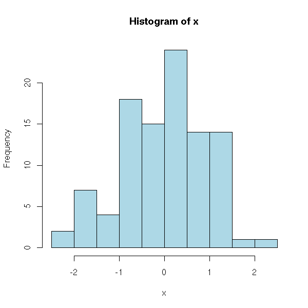
Plot a histogram

x <- rnorm(100)
hist(x, col = "light blue")

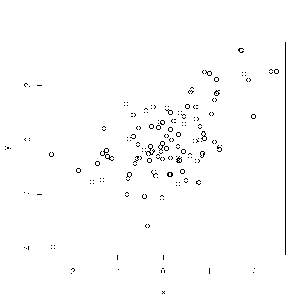
Display a scatter plot of two variables

N <- 100
x <- rnorm(N)
y <- x + rnorm(N)
plot(y ~ x)

Add a "regression line" to that scatter plot.

N <- 100
x <- rnorm(N)
y <- x + rnorm(N)
plot(y ~ x)
abline( lm(y ~ x), col = "red" )

Print a message or a variable

print("Hello World!")

Concatenate character strings

paste("min:        ", min (x$DS1, na.rm=T)))

Write in a file (or to the screen)

cat("\\end{document}\n", file="RESULT.tex", append=TRUE)

This work is licensed under a Creative Commons Attribution-NonCommercial-ShareAlike 2.5 License.

Vincent Zoonekynd
<zoonek@math.jussieu.fr>
latest modification on Sat Jan 6 10:28:14 GMT 2007

Introduction to R

Features

Statistics vs Signal processing

GUI -- or lack thereof

Speed issues

Memory issues

Graphics

Freedom

Examples

Installing R

Windows

MacOS X

Linux

Linux: Installing R on Mandriva

Linux: Installing R on Gentoo

Linux: installing R from the sources

R: Documentation

First steps

RTFM

CRAN Task Views

Graphics

More technical documents

The pictures in the manual

Graphical interface -- R for non-statisticians and non-programmers

ESS

Windows-specific stuff

R Commander

Zelig

SciViews

JGR (pronounce "jaguar")

R: Some elementary functions